TesserAct: Learning 4D Embodied World Models
1. Quick overview of the paper
| What should the paper solve? | Solve the problem of incomplete spatial relationships caused by the embodied world model only predicting the future in 2D pixel space. For tasks such as grabbing, opening drawers, and using tools, robots need depth, surface orientation, and dynamic geometry; generating only RGB videos is prone to errors in object scale, shape, pose, and time consistency. |
|---|---|
| The author's approach | The author does not directly predict expensive 4D point cloud or mesh, but chooses lightweight intermediate representation RGB-DN video. The method includes: automatically constructing RGB, Depth, and Normal annotation data sets; modifying and fine-tuning CogVideoX to generate RGB-DN; using depth-normal integration, optical flow temporal consistency and regularization loss to reconstruct the video into a 4D scene; and finally using 4D point cloud to train the inverse dynamics model for action planning. |
| most important results | On real/synthetic 4D scene generation, TesserAct achieves optimal results on depth, normal and reconstructed point cloud Chamfer $L_1$; among 9 tasks of RLBench action planning, 4DWM exceeds UniPi* and Image-BC on 7 tasks, such as close box 88, open drawer 80, open jar 44, sweep to dustpan 56, water plants 41. |
| Things to note when reading | The key to this paper is not as simple as "predict two more channels", but whether RGB-DN is sufficient as a low-dimensional interface for the 4D world: it must simultaneously retain the trainability of the video model, the availability of geometric reconstruction, and the benefits of downstream action planning. When reading, you should focus on tracking: whether the data annotation is reliable, whether the joint modeling of depth/normal and RGB really improves 4D reconstruction, when geometric information helps action planning, and when 2D information is sufficient. |
Contribution in one sentence
The paper advances the robot video world model from 2D RGB prediction to RGB-DN conditional generation, and proposes a reconstruction and downstream control pipeline from generated video to spatiotemporally consistent 4D scene.
keywords
4D Embodied World Model RGB-DN Video CogVideoX Fine-tuning Depth-Normal Integration Inverse Dynamics
2. Research questions and motivations
2.1 Why 2D world model is not enough
Learned world models aim to simulate environmental dynamics and are used for policy synthesis, data simulation and long-horizon planning. Existing visual world models mostly generate future RGB videos in 2D pixel space, but the physical world is essentially three-dimensional. Looking only at RGB makes the model lack depth, 6-DoF pose, surface orientation and geometric constraints, which is insufficient for robot operation that requires precise position and attitude.
The core problem cited by the author in the Introduction is that 2D models may produce object size and shape inconsistencies over time, resulting in limitations in data-driven simulation and robust policy learning. In other words, just because the generated video looks reasonable does not mean that it can support the robot's judgment of the object's geometry.
2.2 Why not just predict full 4D geometry
Generating 3D scenes directly over time is very expensive, and both training and inference are more complex than 2D video. The trade-off for TesserAct is to predict RGB-DN video: RGB represents appearance, Depth represents geometric distance, and Normal represents surface orientation. This representation is much lower-dimensional than the complete 4D scene, has more geometric information needed by the robot than RGB, and can reuse the ability of existing video diffusion models.
2.3 Data bottleneck
Training a 4D world model requires large-scale video data with depth and normal directions, but real robot data usually does not have these annotations. The author's solution is to extend the existing robot video data to RGB-DN: simulated data uses simulator depth and depth2normal, real data uses RollingDepth to estimate depth, and Temporal-Consistent Marigold-LCM-normal to estimate normal. This automatic annotation pipeline is the prerequisite for the method to be established.
4. Detailed explanation of method
4.1 Task form: conditional RGB-DN video diffusion
The paper writes RGB \(\mathcal{V}\), Depth \(\mathcal{D}\), and Normal \(\mathcal{N}\) video generation as conditional denoising tasks:
Among them, \(\mathbf{v}, \mathbf{d}, \mathbf{n}\) is the latent sequence of RGB, depth and normal in the future, and the condition \(\mathbf{v}^0, \mathbf{d}^0, \mathbf{n}^0, \mathcal{T}\) corresponds to the initial image, initial depth/normal and text action command. For any mode latent \(\mathbf{z}\in\{\mathbf{v}, \mathbf{d}, \mathbf{n}\}\), forward diffusion is:
Splicing the three modalities into \(\mathbf{x}=[\mathbf{v}, \mathbf{n}, \mathbf{d}]\), the denoising network \(\epsilon_\theta(\mathbf{x}_t, t, \mathbf{x}^0, \mathcal{T})\) learns the reverse process and finally decodes it into pixel space.
4.2 RGB-DN data set construction
The 4D embodied video dataset constructed by the author comes from two types of data: synthetic and real. The simulation part selects 20 difficult tasks from RLBench. Each task generates 1000 instances, each instance has 4 perspectives, totaling 80k synthetic 4D embodied videos. RLBench provides metric depth, but not normal, so DSINE's is used depth2normal Estimating normal from depth; to enhance generalization, use Colosseum-style scene randomization to vary the background, desktop texture, and lighting.
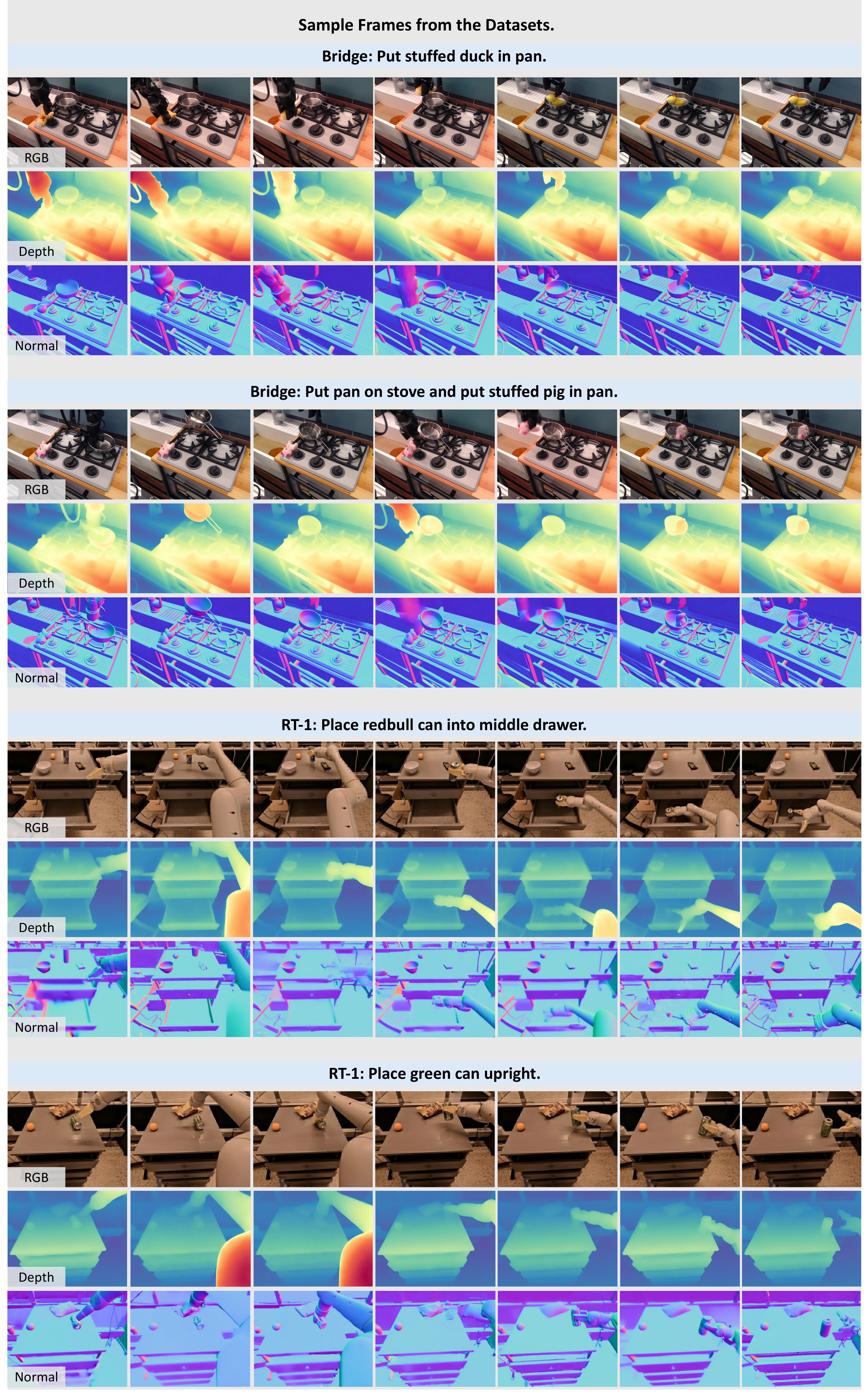
Real data comes from RT1 Fractal and Bridge in OpenX, plus SomethingSomethingV2 is added to increase action/command diversity. Real data lacks depth/normal. The author uses RollingDepth to mark affine-invariant depth and Temporal-Consistent Marigold-LCM-normal to mark normal.
| Dataset | Domain | Depth Source | Normal Source | Embodiment | # Videos |
|---|---|---|---|---|---|
| RLBench | Synthetic | Simulator | Depth2Normal | Franka Panda | 80k |
| RT1 Fractal Data | Real | RollingDepth | Marigold | Google Robot | 80k |
| Bridge | Real | RollingDepth | Marigold | WidowX | 25k |
| SomethingSomethingV2 | Real | RollingDepth | Marigold | Human Hand | 100k |
4.3 Model architecture: from CogVideoX to RGB-DN predictor
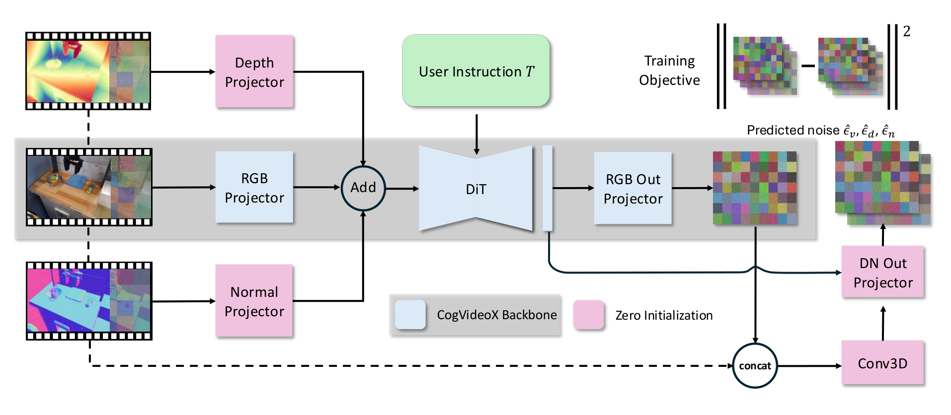
Instead of training a diffusion video model from scratch, TesserAct modifies and fine-tunes CogVideoX. RGB, depth, and normal videos are encoded by CogVideoX's 3D VAE respectively, and VAE does not require additional fine-tuning. The input side introduces independent projectors for the three modes:
The text condition \(\mathcal{T}\) is defined as an action instruction plus the robot name, such as "pick up apple google robot", in order to distinguish different embodiments. The output side retains the original RGB output mode \(\epsilon^*_\mathbf{v}=\texttt{OutputProj}(h)\), and then adds a module for depth/normal: use Conv3D to encode the splicing of latent input and RGB denoised output, and then combine it with DiT hidden states to obtain the denoising prediction of depth/normal through DNProj.
In order to retain the RGB generation knowledge of CogVideoX, the author initializes the backbone with CogVideoX weights, and initializes other new modules with 0, so that the RGB output in the early stage of training is consistent with CogVideoX. The training loss is the MSE of the tri-modal noise prediction:
4.4 Reconstruct 4D scene from RGB-DN video
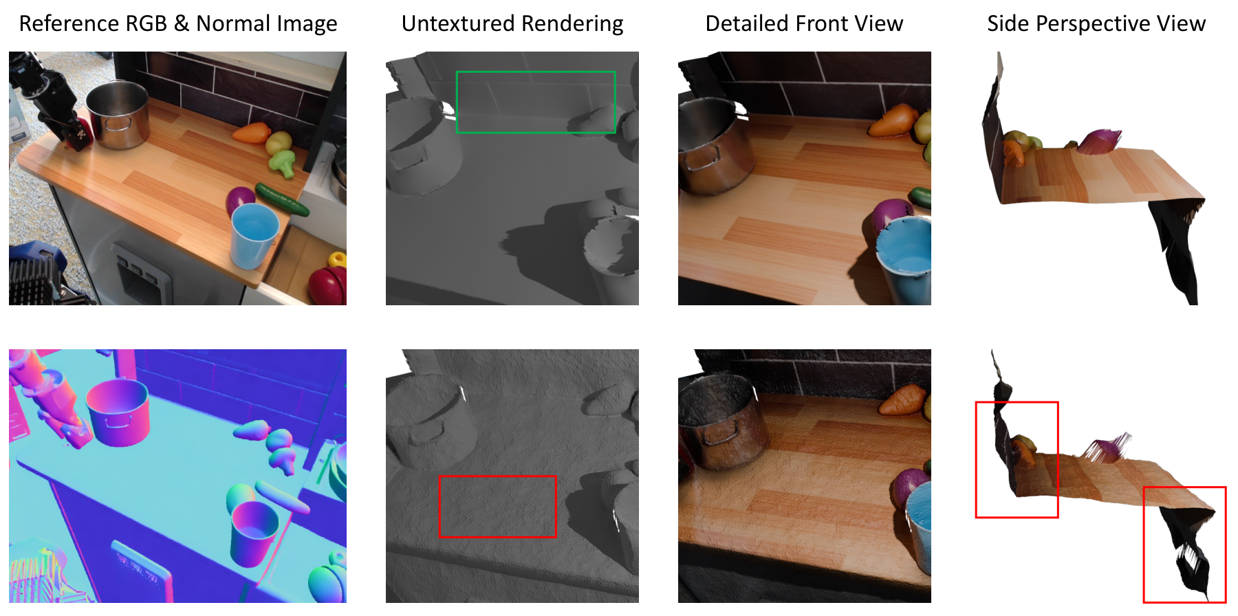
The generated depth is a relative depth and cannot directly obtain a 3D scene with the same complete scale; and only frame-by-frame depth-normal integration lacks temporal consistency. TesserAct's reconstruction algorithm first uses normal map to optimize the depth of each frame, and then uses optical flow to establish cross-frame constraints.
Under the perspective camera, pixel \(\boldsymbol{u}=(u, v)^T\), depth \(d\), and normal \(\boldsymbol{n}=(n_x, n_y, n_z)\) satisfy the normal integration constraint of log-depth \(\tilde{d}=\log(d)\). The author uses iterative optimization form:
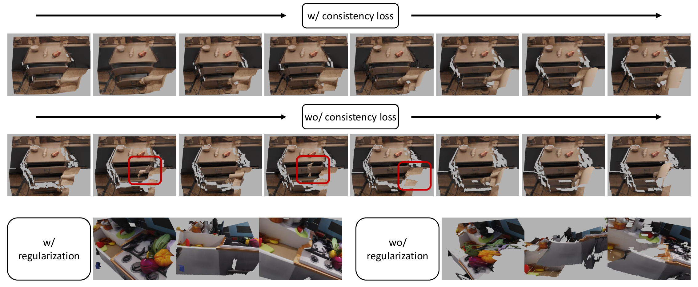
Then use RAFT optical flow \(\mathcal{F}\) to identify static and dynamic regions: \(\mathcal{M}_s^i=\|\mathcal{F}^i\|\le c\), \(\mathcal{M}_d^i=\neg\mathcal{M}_s^i\), and the background region is \(\mathcal{M}_b^i=\mathcal{M}_s^i\cap\mathcal{M}_s^{i-1}\). According to flow, depth warp the previous frame to the current frame position and define temporal consistency loss:
At the same time, regularization loss is added to prevent the optimized depth from deviating too far from the generated depth:
The overall goal is:
4.5 Use 4D scene for embodied action planning
After generating the 4D scene, the author trained the inverse dynamics model and output a 7-DoF action based on the current state \(s_i\), predicted future state \(s_{i+1}\) and instruction \(\mathcal{T}\):
In the specific implementation, PointNet encodes the 3D features of the 4D point cloud, then splices it with the instruction text embedding, and outputs the action through MLP. The goal of this downstream experiment is to verify that the geometric information reconstructed by RGB-DN is not only more beautiful in visualization, but can actually help the robot action decision-making.
5. Experiments and results
5.1 4D scene prediction settings
4D scene prediction is evaluated in both real and synthetic domains. Real domain uses 400 unseen samples of RT1 Fractal and Bridge, and depth/normal is estimated according to the data construction process; Synthetic domain uses 200 unseen samples of RLBench, and depth/normal can be obtained directly from the emulator. Each sample was generated 10 times and the average is reported.
The indicators are divided into four categories: FVD, SSIM, and PSNR for RGB quality; AbsRel, \(\delta_1\), and \(\delta_2\) for depth; Mean, Median, and \(11.25^\circ\) for normal; and Chamfer \(L_1\) for point cloud reconstruction. Baselines include OpenSora, CogVideoX, and the author's implementation of 4D Point-E.
5.2 4D scene generation main results
| Domain | Method | RGB FVD ↓ | RGB SSIM ↑ | RGB PSNR ↑ | Depth AbsRel ↓ | Normal Mean ↓ | Chamfer L1 ↓ |
|---|---|---|---|---|---|---|---|
| Real | 4D Point-E | - | - | - | - | - | 0.2211 |
| Real | OpenSora | 23.67 | 71.31 | 19.25 | 31.41 | 41.82 | 0.3013 |
| Real | CogVideoX | 20.64 | 79.38 | 22.39 | 26.17 | 19.53 | 0.2191 |
| Real | TesserAct | 21.59 | 75.86 | 20.27 | 22.07 | 15.74 | 0.2030 |
| Synthetic | 4D Point-E | - | - | - | - | - | 0.1086 |
| Synthetic | OpenSora | 54.11 | 65.90 | 19.28 | 18.40 | 12.94 | 0.2570 |
| Synthetic | CogVideoX | 41.23 | 76.60 | 20.87 | 19.81 | 20.36 | 0.2884 |
| Synthetic | TesserAct | 40.01 | 77.59 | 19.73 | 16.02 | 14.75 | 0.0811 |
There are two levels to distinguish when reading this table: TesserAct may not necessarily surpass CogVideoX in all RGB indicators, especially the RGB FVD/SSIM/PSNR of real domain is still the best of CogVideoX; but TesserAct is the strongest in depth, normal and final point cloud Chamfer. The proposition of the paper is exactly this: sacrificing or maintaining similar RGB quality in exchange for more reliable 4D geometry.
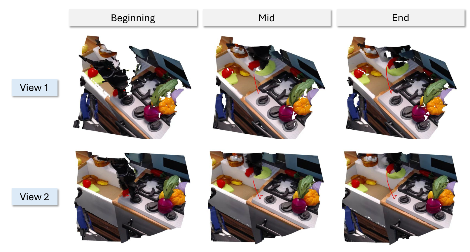
5.3 Novel view synthesis
The author further tested novel view synthesis after monocular video to 4D. On RLBench, enter the front camera monocular video and compare the overhead and left shoulder camera perspectives. Baseline is Shape of Motion, a video reconstruction method based on Gaussian Splatting.
| Method | PSNR ↑ | SSIM ↑ | LPIPS ↓ | CLIP Score ↑ | CLIP Aesthetic ↑ | Time Costs ↓ |
|---|---|---|---|---|---|---|
| Shape of Motion | 10.94 | 24.02 | 73.82 | 66.67 | 3.61 | about 2 hours |
| TesserAct | 12.99 | 42.62 | 60.51 | 83.02 | 3.73 | approx. 1 min |
The key point of this result is speed: TesserAct's 4D representation avoids slow per-scene optimization and is also better in PSNR, SSIM, CLIP Score and aesthetics. However, Shape of Motion is better in the LPIPS table, which shows that TesserAct's visual perception distance is not dominant in all indicators.
5.4 Embodied action planning
Action planning is evaluated on 9 challenge tasks of RLBench, with 100 episodes of average success rate reported for each task. Baselines are Image-BC and UniPi*. UniPi* was reimplemented by the author and uses fine-tuned CogVideoX as backbone for fair comparison.
| Method | close box | open drawer | open jar | open microwave | put knife | sweep to dustpan | lid off | weighing off | water plants |
|---|---|---|---|---|---|---|---|---|---|
| Image-BC | 53 | 4 | 0 | 5 | 0 | 0 | 12 | 21 | 0 |
| UniPi* | 81 | 67 | 38 | 72 | 66 | 49 | 70 | 68 | 35 |
| 4DWM / TesserAct | 88 | 80 | 44 | 70 | 70 | 56 | 73 | 62 | 41 |
The results show that geometric information is helpful for most tasks, especially close box, open jar, sweep to dustpan, water plants and other tasks that require object geometry, tool usage or precise spatial relationships. The paper also honestly points out that TesserAct is not as good as UniPi* in open microwave and weighing off, probably because the 2D front image of these tasks already provides enough information, and additional 3D processing does not necessarily bring benefits.
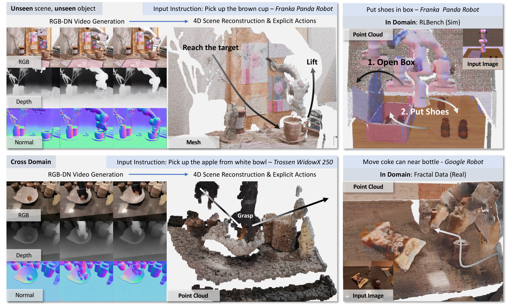
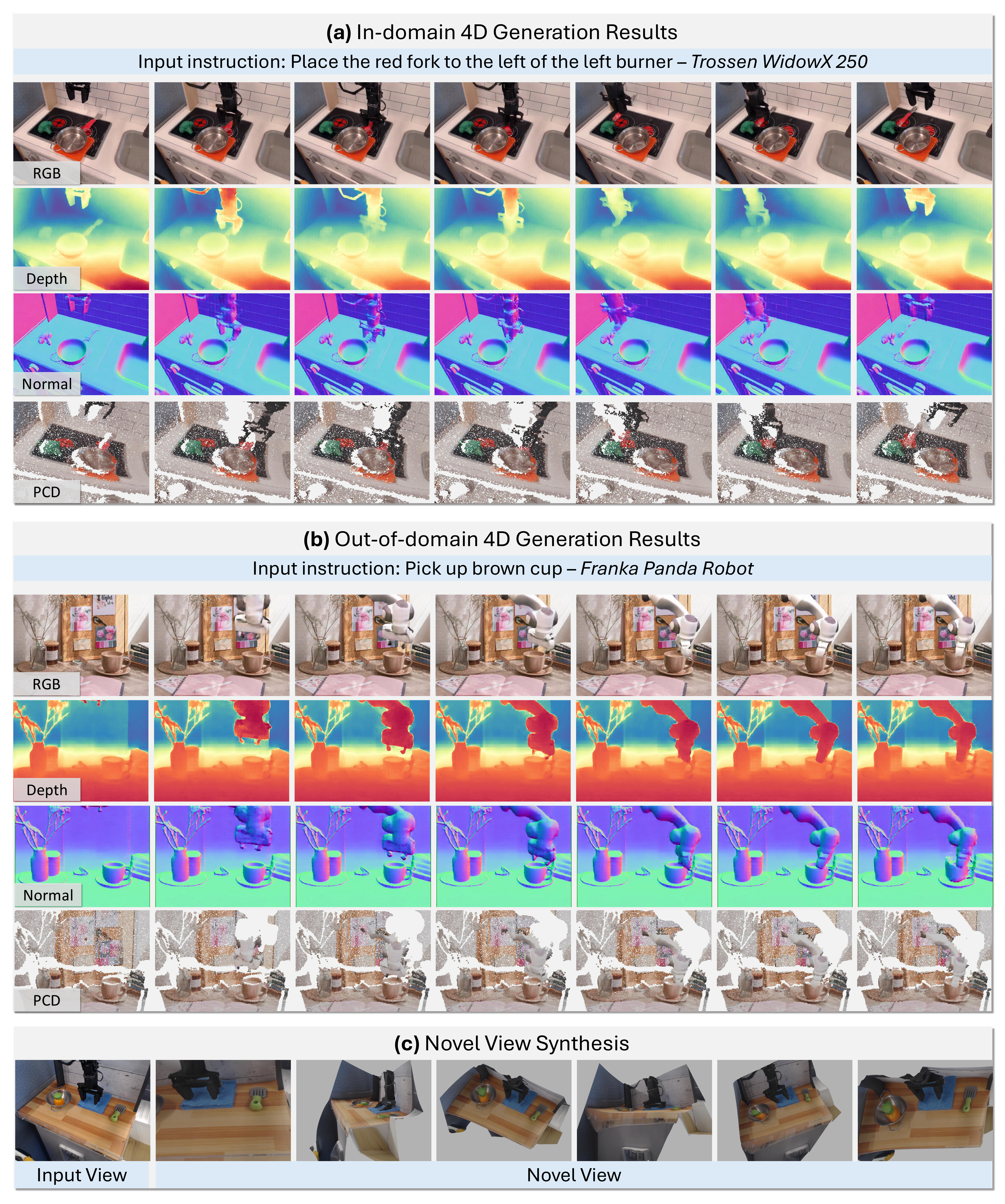
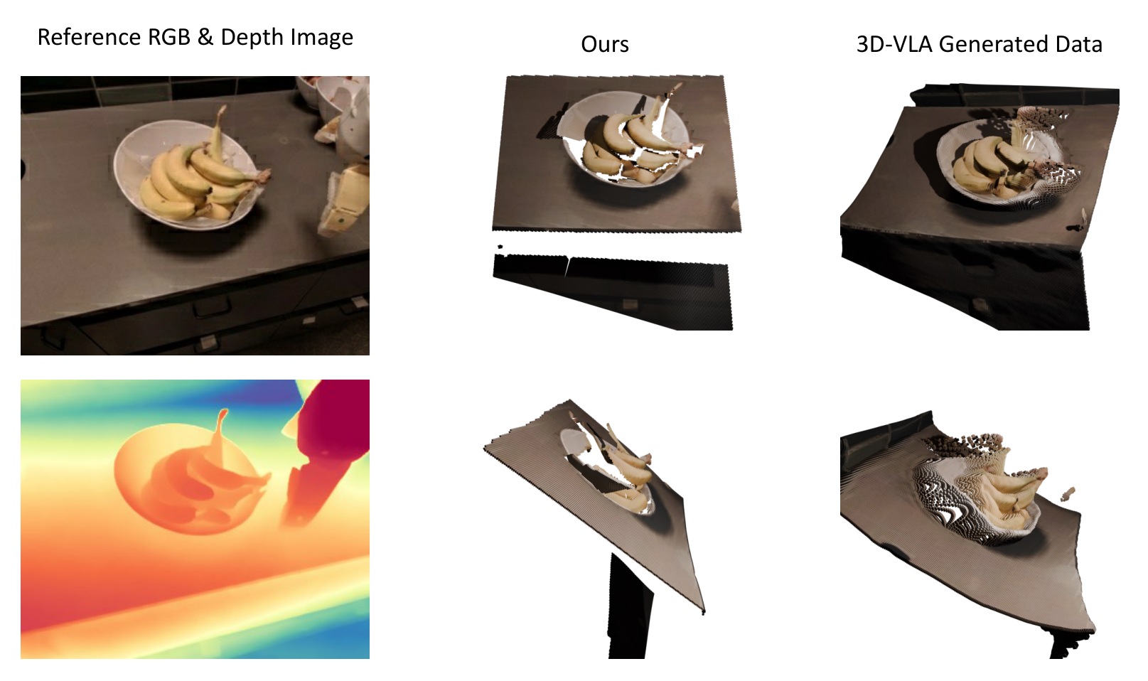
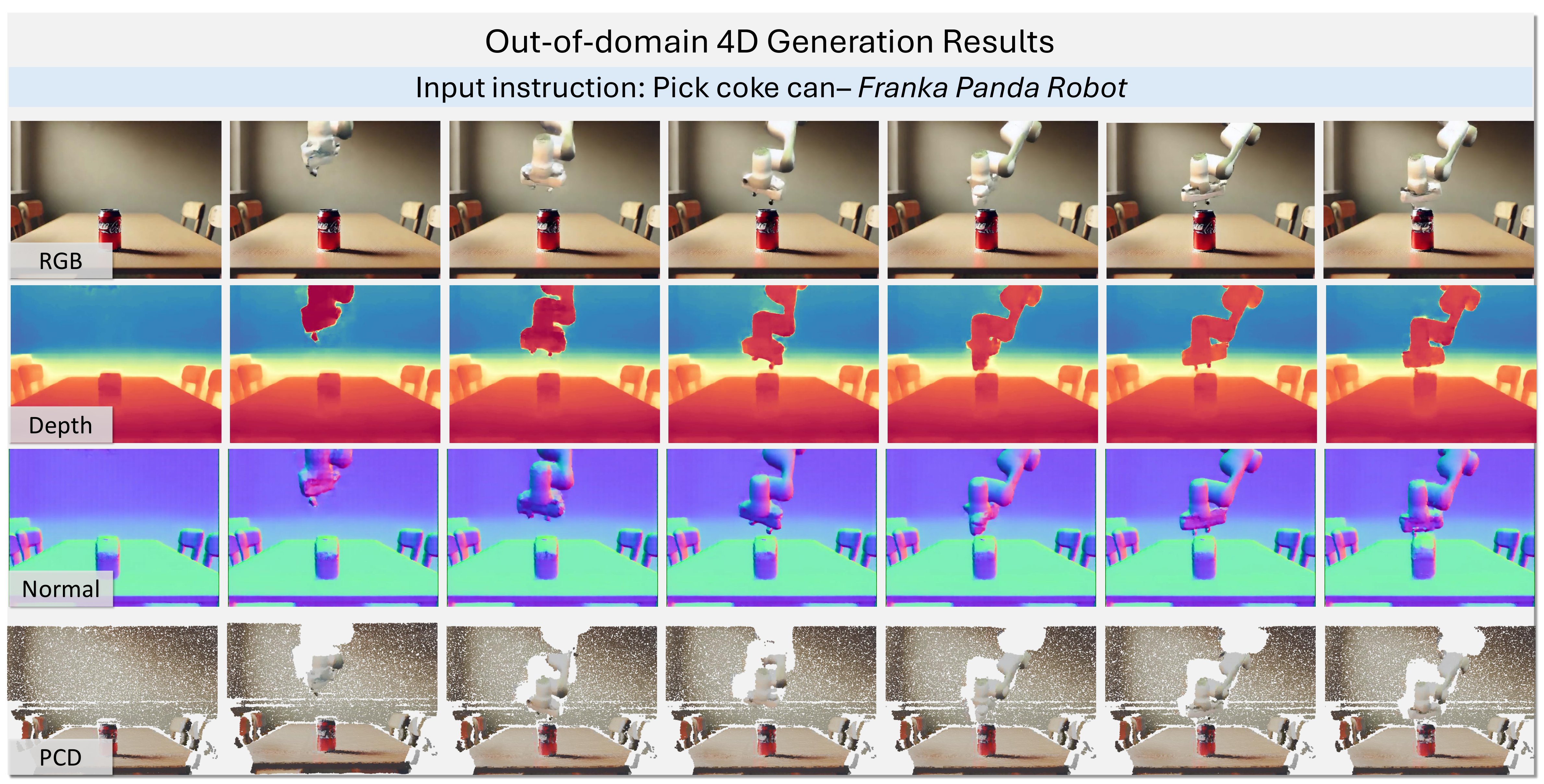
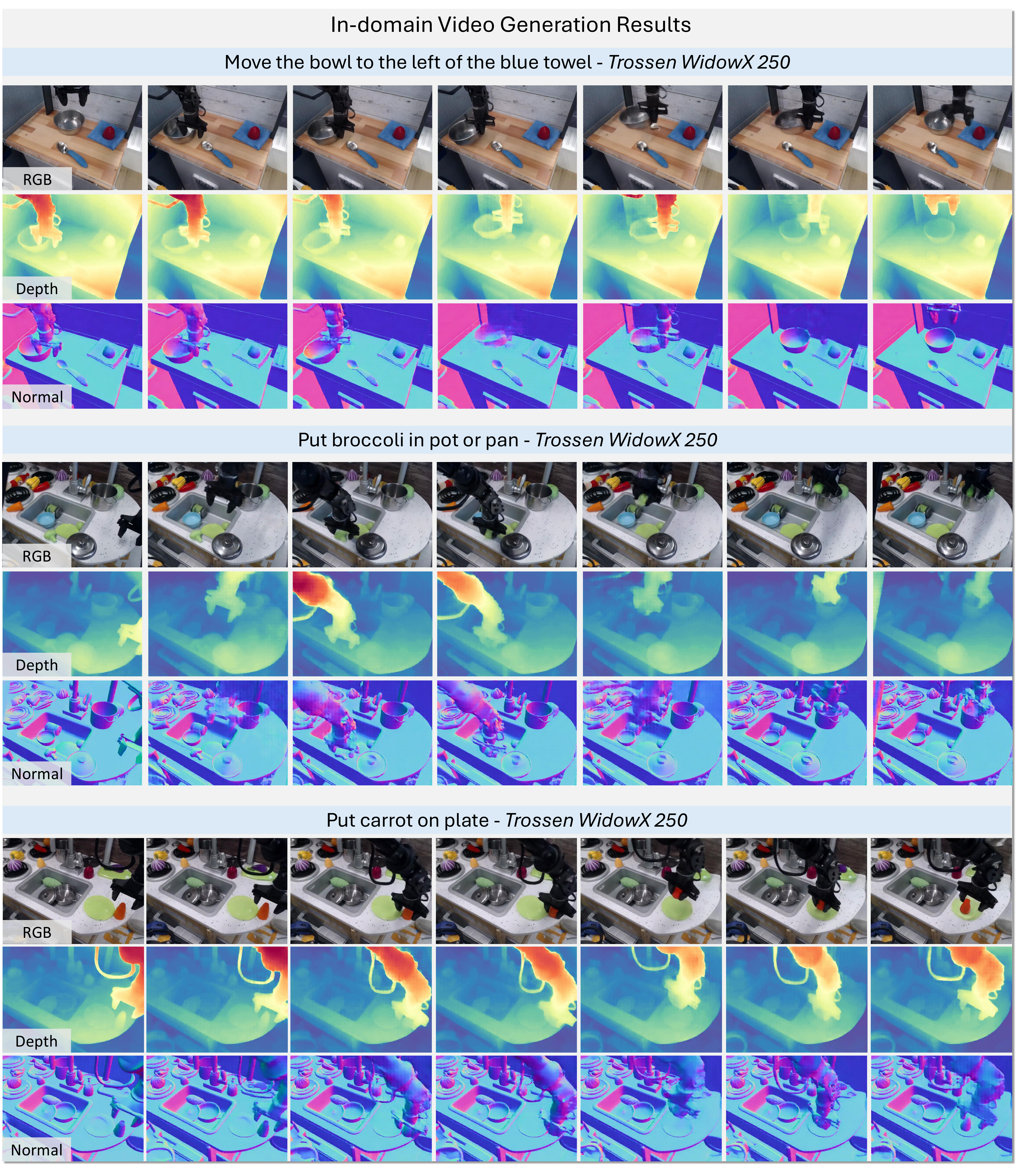
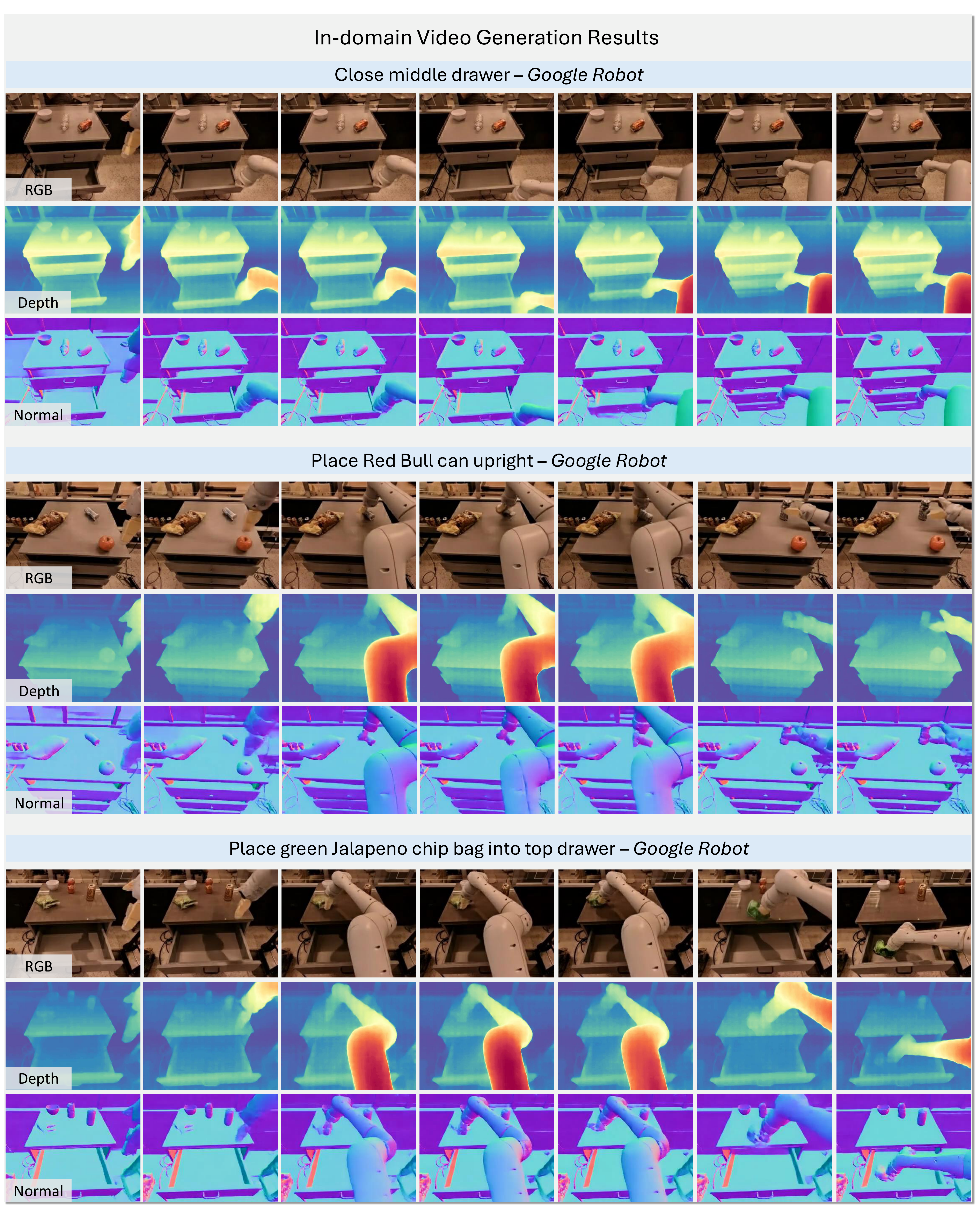
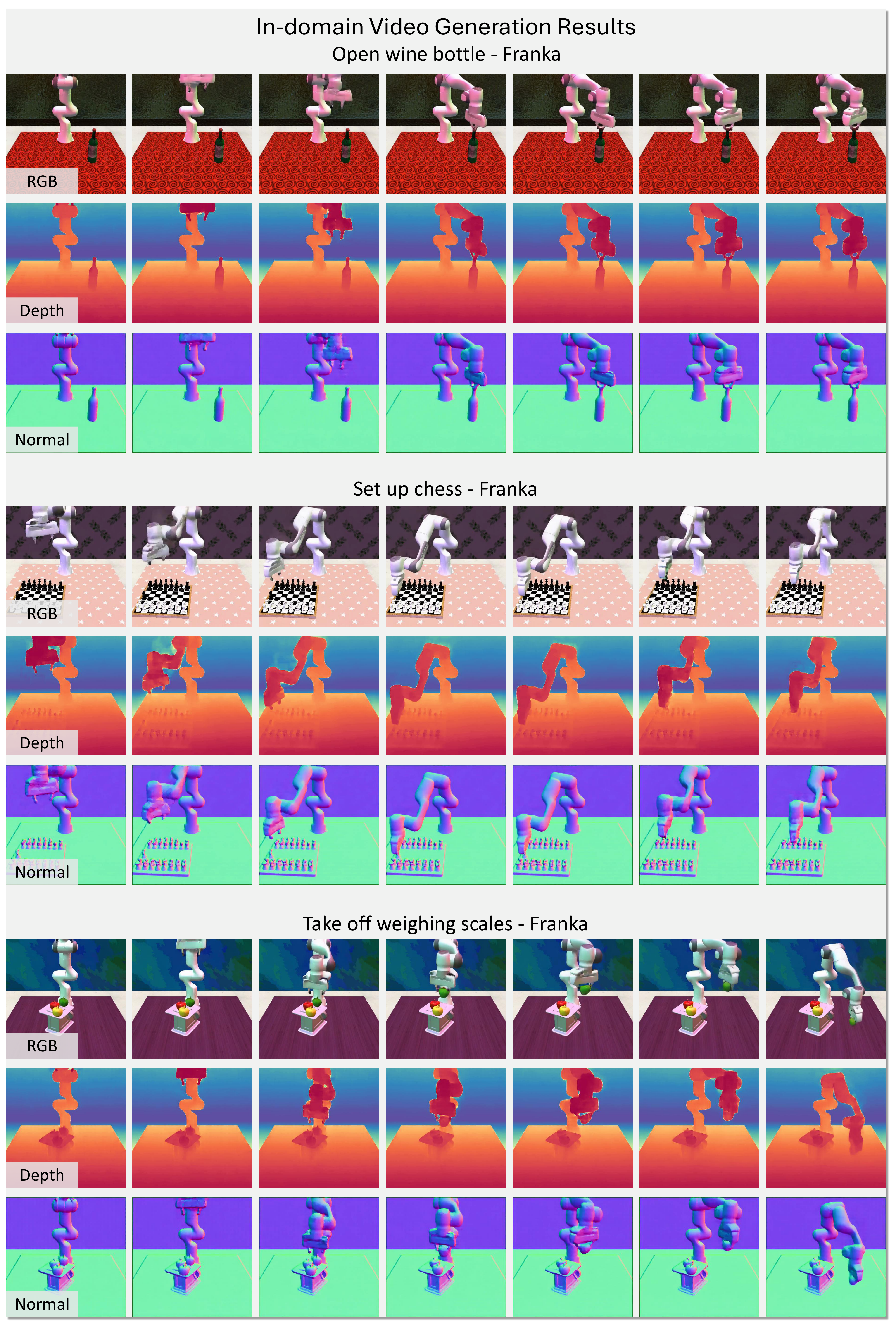
5.5 Supplementary material Qualitative results
The supplementary material adds data annotation, out-of-domain generation, RGB-DN video generation for each dataset, and explicit action trajectory visualization. They do not change the main conclusion, but help determine the scope of applicability and risk of failure of the method.
6. reproducibility Key Points
6.1 Video diffusion model training
[Supplementary material Implementation Details] The model is based on CogVideoX. Depth/normal projector and RGB projector use the same architecture; output side Conv3DNet There are 3 layers, MLP has 2 layers, and the dimensions are both 1024. The model outputs 49 frames, using gradient checkpointing, global batch size 16, and bf16 precision. Sampling uses DDPM scheduler 50 steps, classifier-free guidance scale is 7.5.
Training 40, 000 iterations, initial learning rate \(1\times10^{-4}\), gradient clipping 1.0, warmup 1, 000 steps. The optimizer is Adam, \(\epsilon=1\times10^{-15}\), EMA decay 0.99.
6.2 4D scene generation hyperparameters
[Supplementary material 4D Scene Generation] The reconstruction loss parameters are adjusted according to different data sets:
| Dataset | \(\lambda_d\) | \(\lambda_b\) | \(\lambda_{g1}\) | \(\lambda_{g2}\) |
|---|---|---|---|---|
| RT-1, Bridge | 20 | 200 | 20 | 20 |
| RLBench | 20 | 200 | 2 | 2 |
The author clearly stated that these \(\lambda\) will change with the scene, and the actual best performance requires parameter adjustment. This is critical when reproducing because the quality of the 4D reconstruction depends not only on the generated model but also on the post-processing optimization weights.
6.3 Robotics planning training
In RLBench planning, the main difference of the model is that it is changed to 13 frames and fine-tune, and the fixed resolution is 512 × 512. Each task collects 500 samples to train the inverse dynamics model. During inference, all future keyframes are first predicted and recorded, and then only the inverse dynamics model is queried, and actions are output based on the current state and the predicted future state.
[Supplementary material Implementation Details for Robotics Planning] The Action prediction stage first filters the background and ground, retains only point clouds related to the desktop and the operated object, and then samples 8192 points. PointNet extracts point cloud features, concatenates them with instruction language embedding, inputs 4-layer MLP, and outputs 7-DoF actions. To adapt the video diffusion model output, the author adds Gaussian noise with a relative amplitude of 20% to the image and point cloud coordinates.
6.4 Recurrence risk list
- Automatic labeling error: The depth and normal of real data come from off-the-shelf estimators, not ground truth; the estimator bias is passed into the world model.
- Multimodal alignment: RGB, Depth, and Normal must be consistent in time, otherwise the reconstructed 4D scene will be misaligned in the dynamic area.
- Reconstruct hyperparameters: \(\lambda\) is different for different data sets. The paper also states that parameters need to be adjusted, and these settings must be reported in replication experiments.
- Control closed loop details: In the future, the selection of keyframes, the state correspondence method of inverse dynamics, and point cloud filtering rules will all affect the success rate of RLBench.
- Computing power depends on: Fine-tuning CogVideoX, generating 49-frame RGB-DN video, and evaluating multiple samples all have high memory and time costs.
7. Analysis, Limitations and Boundaries
7.1 The most valuable part of this paper
The most valuable part is that it proposes a very practical 4D world model representation: RGB-DN video. It's not the most complete 4D representation, but it's nicely stuck between "trainable by existing video models" and "enough to reconstruct the geometry needed for the robot". For embodied AI, this intermediate representation is more geometrically constrained than directly generating RGB videos, and is easier to train at scale than directly generating dynamic point clouds or meshes.
The second value point is that the paper connects the quality of the world model and downstream action planning. The 4D scene generation table proves that depth/normal/Chamfer is better, and the RLBench action planning table further shows that geometry improvement can translate into success rate gains in most tasks. This is more convincing than just showing a nice 4D visualization.
7.2 Why the results hold up
The results are tenable mainly because the evidence chain is relatively complete. First, the paper evaluates 4D scenes in both real and synthetic domains. Synthetic RLBench has ground-truth depth/normal, which can more objectively verify geometric quality. Second, the indicators cover RGB, depth, normal and point cloud, and do not just rely on a single visual indicator. Third, novel view synthesis and action planning verify the practicality of 4D representation from reconstruction applications and robot control applications respectively. Fourth, the supplementary material gives training hyperparameters, reconstruction weights, point cloud filtering, and action model details so that the method is not completely black box.
However, caution is needed: the depth/normal annotation on real data comes from the estimator, so the "true value" of the real-domain depth/normal indicator also has an estimation chain; RLBench action planning is a simulation environment, and real robot closed-loop control has not yet formed quantitative evidence of the same strength.
7.3 Clear limitations of the paper
The authors make it clear in Limitations: RGB-DN means cheap and predictable, but only captures a single surface of the world. To build a more complete 4D world model, in the future, the generated model can generate multiple RGB-DN views and then integrate them into a more complete 4D scene.
7.4 Additional boundaries and possible improvements
- Single-view occlusion problem: It is difficult for a single RGB-DN sequence to recover the geometry behind occluded objects, and multi-view generation or active view selection would be stronger.
- Estimator dependencies: The quality of RollingDepth and Marigold directly affects real data annotation. If the estimator fails after domain change, world model training will also be contaminated.
- Geometry is not always necessary: The 2D baseline is stronger in open microwave and weighing off, indicating that not all tasks benefit from 4D.
- Insufficient dynamic contact modeling: RGB-DN representation can reconstruct surfaces and motions, but physical variables such as contact forces, friction, and internal states of objects are still not explicitly modeled.
- Engineering complexity: The method requires multiple modules such as video generation, depth/normal annotation, optical flow, depth optimization, point cloud filtering, and inverse dynamics, any of which may become a deployment bottleneck.
8. Preparation for group meeting Q&A
Q1: What is the essential difference between TesserAct and ordinary video world model?
Ordinary video world model mainly predicts RGB future frames; TesserAct simultaneously predicts RGB, depth and normal, and then reconstructs 4D point clouds. It advances the output of the world model from "looking like the future" to "containing a future that can be used for geometric reasoning".
Q2: Why choose RGB-DN instead of directly generating point cloud?
Directly generating dynamic point clouds is more expensive for training and inference, and the number of frames is limited. RGB-DN video is compatible with existing video diffusion models and has lower data dimensions while retaining the depth and surface orientation required to reconstruct 3D scenes.
Q3: Which group of formulas is the most core in this paper?
One group is RGB-DN conditional denoising objective, which explains how the model jointly generates three-modal video; the other group is \(\mathcal{L}_s+\mathcal{L}_c+\mathcal{L}_r\) of 4D scene reconstruction, which explains how to use normal, optical flow and generated depth to obtain consistent depth in space and time.
Q4: What is the most convincing result in the experiment?
In the 4D scene table, Chamfer \(L_1\) is the best in both real and synthetic, indicating that the reconstructed geometry is indeed better; in RLBench action planning, 7/9 tasks exceed UniPi*, indicating that geometric advantages can be converted into control benefits.
Q5: What should be questioned most?
The depth/normal of real data is not ground truth, but estimator annotation; in addition, downstream action planning is mainly verified in RLBench simulation. To prove that it is a universal robot world model, stronger real robot closed-loop experiments and multi-view/occlusion scene evaluation are needed.