Unified 4D World Action Modeling from Video Priors with Asynchronous Denoising

Method name: X-WAM

Authors: Jun Guo, Qiwei Li, Peiyan Li, Zilong Chen, Nan Sun, Yifei Su, Heyun Wang, Yuan Zhang, Xinghang Li, Huaping Liu

Organization: Tsinghua University, Xiaomi Robotics, Peking University, CASIA

Publication: arXiv preprint, 2026; the source code is NeurIPS 2026 preprint template, the arXiv page is not marked with formal receipt information

Version: v2, 2026-05-07; first version 2026-04-29

Links: arXiv 2604.26694 | PDF | Project

Contents

1. Quick overview of the paper
2. Motivation
3. Summary of related work
4. Detailed explanation of method
5. Experiment
6. Summary of recurrence information
7. Analysis, Limitations and Boundaries

1. Quick overview of the paper

One-sentence summary: X-WAM puts robot strategy execution, future multi-view RGB-D video generation and 3D/4D reconstruction into the same diffusion world-action model, uses a lightweight depth branch to add spatial modeling, and uses Asynchronous Noise Sampling while maintaining action decoding efficiency and video generation quality.

Difficulty rating: ★★★★★. Need to understand video diffusion/DiT, flow matching, world action model, RGB-D/multi-view geometry, robot imitation learning and asynchronous sampling reasoning.

Keywords: World Action Model4D World ModelingRGB-D GenerationAsynchronous Noise SamplingRobotic Foundation Model

Reading targeting item	content
What should the paper solve?	Existing unified world action models mainly stay in 2D pixel-space, lacking explicit 3D spatial awareness; at the same time, actions need to be low-latency, and video/world generation needs to be high-quality, and the two sampling step requirements conflict.
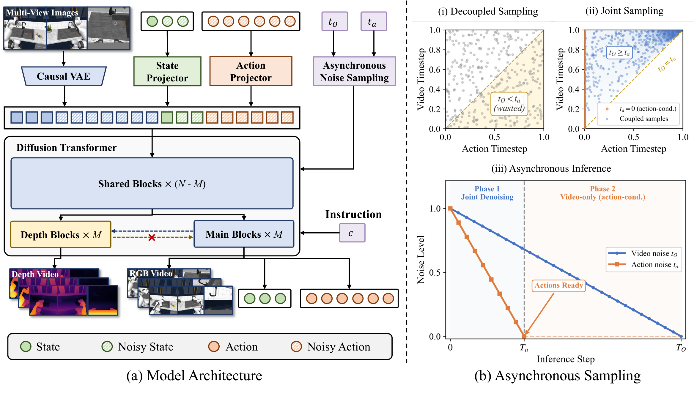
The author's approach	Initialized from Wan2.2-TI2V-5B video DiT, jointly predict future RGB, depth, state and action; copy the last $M$ DiT blocks to construct a depth branch; use ANS to make the training noise distribution match asynchronous inference.
most important results	The average SR of RoboCasa is 79.2%, and RoboTwin 2.0 clean/randomized is 89.8%/90.7%; RoboCasa 4D reconstruction exceeds the comparison method in RGB, depth and point cloud indicators.
Things to note when reading	The core is not just "adding depth", but how to put depth, action and video into a unified denoising sequence without destroying the pre-trained video prior or significantly increasing action latency.

Core contribution list

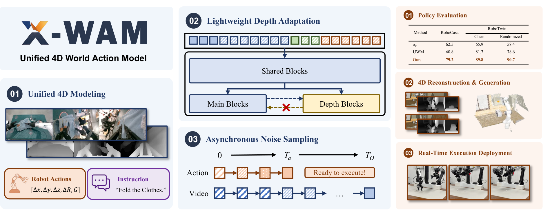
Proposed unified 4D World Action Model X-WAM.One framework simultaneously serves video generation, 3D reconstruction, policy success and efficient action execution.
Propose lightweight depth adaptation.The depth prediction branch is formed by copying the DiT rear block, and the depth branch reads the main branch in one direction to preserve the distribution and parameter integrity of the pre-trained video backbone as much as possible.
Proposed Asynchronous Noise Sampling.During training, samples are taken from the joint distribution that satisfies $t_O\ge t_a$. During inference, the action is quickly decoded with fewer steps, and the video continues to be completely denoised.
Large-scale pre-training and multi-layer verification.Pretrained on 5, 873.9 hours, 1, 492, 026 episodes of robot data, and evaluated on RoboCasa, RoboTwin 2.0, 4D reconstruction, and real dual-arm robot tasks.

2. Motivation

2.1 What problem should be solved?

The paper divides the current route of embodied AI into two categories: policy models and world models. VLA/policy models are good at instruction following and action prediction, but lack the geometric intuition and physical awareness of how actions continuously unfold in the real world; world models can simulate future observations, but usually cannot directly output executable actions. Recent WAM/UWM attempts to unify video generation and action prediction, but still mainly work in 2D pixel-space.

The author believes that the real physical world is essentially three-dimensional; only doing 2D pixel prediction will lose the geometric structure, so that the model may generate a physically unreasonable future, and it is difficult to perform geometrically faithful 3D reconstruction.

2.2 Limitations of existing methods

VLA: Ability to move from language and vision to action, but explicit spatial modeling is weak, especially tasks requiring fine interpolation, long-term progression understanding, and geometric reasoning.
World models: Can generate future observations, but does not directly generate executable robot actions.
Existing unified WAM/UWM: Started to combine video/action, but it is limited to 2D pixel-space and lacks explicit 3D spatial awareness.
Asynchronous sampling previous work: For action latency, video/action timestep will be decoupled; if each modal timestep is sampled independently during training, $t_O will be generated that will not appear during testing.

2.3 The solution ideas of this article

The high-level idea of X-WAM is to extend robot observation to multi-view RGB-D future generation based on the strong visual prior of the pre-trained video diffusion model; depth uses lightweight branch adaptation instead of rebuilding the entire model; action and video share a unified denoising framework, but through ANS, the action completes denoising first and the video continues denoising.

3. Summary of related work

3.1 Related work of the thesis self-description

Technical line	How to position the paper	The difference between X-WAM
Unified World Action Modeling	UWM, Motus, VideoVLA, Genie Envisioner, etc. put video generation and action prediction into a framework; DreamZero, LingBot-VA, GigaWorld-Policy, etc. use causal masks, KV caching or timestep decoupling to reduce latency.	X-WAM further adds explicit spatial information and points out that independent timestep sampling does not match the asynchronous inference distribution.
3D Modeling in Embodied Models	One type uses 3D features as target/supervision in VLA; the other type uses point cloud/3D representations directly. World model orientation uses 3D supervision, multi-view consistency, 3DGS or feed-forward reconstruction models.	X-WAM introduces explicit 3D information into unified world action modeling, and simultaneously performs video generator, 3D reconstruction system and policy model in one model.

3.2 Direct comparison with previous works

Dimensions	VLA policy	UWM / WAM	3D world models	X-WAM
Core idea	From vision-language observation to motor command.	Combine future video and action.	Emphasis on 3D representation or reconstruction.	Unify future RGB-D video, state, action, and 4D reconstruction.
key assumptions	Pre-trained VLM/VLA representations are transferable to robot control.	Video prior can improve physical understanding and generalization.	Explicit geometry improves spatial reasoning.	Video prior + lightweight depth adaptation + ANS achieves simultaneous geometric, generative and control gains.
Main limitations	Insufficient awareness of geometric/physical unfolding.	Mostly in 2D pixel-space, or timestep distribution mismatch.	Real-time actions may not necessarily be output directly.	There is still a fixed context and higher latency, which the author clearly states in Limitations.
Experimental comparison	$\pi_0$, $\pi_{0.5}$, GR00T-N1.5, XR-0.	UWM, DreamZero, Cosmos Policy, Motus, GigaWorld-Policy.	Robot4DGen, DreamZero+DA3, X-WAM w/o depth+DA3.	RoboCasa 79.2, RoboTwin randomized 90.7, real earphone packing most settings are higher than XR-0.

4. Detailed explanation of method

4.1 Method overview

The inputs are language instructions $c$, initial proprioceptive state $s_0$, and multi-view initial RGB observations $O_0$. The models jointly predict future RGB videos $O_{1: H}$, depth videos $D_{1: H}$, future states $s_{1: H}$ and actions $a_{1: K}$. In the paper setting, given 1 conditioning RGB frame and 1 initial state, predict $H=8$ future RGB frames, $H=8$ future states, $K=32$ future actions; the action frequency is $K/H=4\times$ of the video frame rate.

Figure 1: X-WAM overview. The top shows the unified modeling of multi-view RGB-D future + action; the bottom shows benchmark, 4D reconstruction and real robot deployment results.

Figure 2: X-WAM framework. On the left is the unified denoising sequence and interleaved depth branch; on the right is the training/inference noise schedule of ANS.

4.2 Method evolution

VLA / policy model → WAM/UWM → X-WAM. The first step starts with directly predicting actions; the second step combines future video generation and action prediction; X-WAM then introduces RGB-D/4D spatial reconstruction, and uses ANS to handle the conflict between action latency and video quality.

4.3 Core design and mathematical derivation

4.3.1 Unified denoising sequence

In plain English: Convert conditional observations, future videos, initial/future states, and future actions into tokens/latent, put them into a sequence, and process them with the same DiT.

$$\mathbf{Z}=[\mathbf{z}_{O_0}, \, \mathbf{z}_{O_{1: H}}, \, \mathbf{z}_{s_0}, \, \mathbf{z}_{s_{1: H}}, \, \mathbf{z}_{a_{1: K}}].$$

$\mathbf{z}_{O}$	RGB video latent, obtained from the original causal VAE encoder $\mathcal{E}$.
$\mathbf{z}_s$	The proprioceptive state is latent after being projected by learnable $\mathrm{MLP}_s$.
$\mathbf{z}_a$	The latent of action after being projected by learnable $\mathrm{MLP}_a$.
$H, K$	Video/state horizon and action horizon; in paper $H=8, K=32$.

The initial observation $\mathbf{z}_{O_0}$ and the initial state $\mathbf{z}_{s_0}$ are fixed during the denoising process, and the timestep is set to $t=0$, which is used as a clean condition.

4.3.2 Wrist camera pose derivation

In plain English: Dynamic wrist camera does not directly predict external parameters, but is derived from end-effector pose and fixed hand-eye calibration.

$$\mathbf{T}_{\text{wrist}}=\mathbf{T}_{\text{ee}}\cdot\mathbf{T}_{\text{h2e}}.$$

$\mathbf{T}_{\text{ee}}\in SE(3)$ is the end-effector pose, and $\mathbf{T}_{\text{h2e}}$ is the fixed hand-to-eye calibration matrix. In this way, multi-view RGB-D fusion can take advantage of robot structural constraints without having to use additional camera extrinsics/ray maps as tokens.

4.3.3 Lightweight Depth Adaptation

In plain English: The first $N-M$ layer shares the video DiT trunk, and the second $M$ layer copies the depth branch; the depth branch reads the main branch in one direction, and the main branch is not reversely affected by the depth token.

$$\mathbf{Z}_D^{(j)}=\mathrm{DepthBlock}_j(\mathbf{Z}_D^{(j-1)}\mid\mathbf{Z}_{\text{m}}^{(j-1)}), \quad \mathbf{Z}_{\text{m}}^{(j)}=\mathrm{DiTBlock}_{N-M+j}(\mathbf{Z}_{\text{m}}^{(j-1)}).$$

$N$	Total number of original DiT blocks.
$M$	Copied as the last block number of the depth branch; the appendix gives $M=10$.
$\mathbf{Z}_D^{(j)}$	The $j$th depth branch hidden state.
$\mathbf{Z}_{\text{m}}^{(j)}$	main branch hidden state.

The depth map is copied three times as pseudo-RGB, encoded/decoded with the same causal VAE; the depth branch predicts inverse depth, and supervised by MSE. This design avoids doubling the attention cost of sequence concatenation, and also prevents channel concatenation from changing the pre-training input distribution.

4.3.4 Asynchronous Noise Sampling

Vernacular: During training, only noise combinations consistent with asynchronous reasoning are sampled: video noise is not less than action noise, that is, $t_O\ge t_a$.

$$ (t_O, t_a)\sim\begin{cases}t_a=0, \; t_O\sim U(0, 1)&\text{w.p. }p, \\ t_a\sim U(0, 1), \; t_O=t_a+(1-t_a)b, \; b\sim \mathrm{Beta}(1.5, 1)&\text{w.p. }1-p.\end{cases} $$

The first situation corresponds to action-conditioned video generation: the action is clean and the video is still being denoised. The second case corresponds to asynchronous joint generation: because $b\in[0, 1]$, so $t_O=t_a+(1-t_a)b\in[t_a, 1]$ naturally satisfies $t_O\ge t_a$.

Supplementary derivation: why this sampling covers the asynchronous inference distribution

In asynchronous reasoning, the action is denoised first using the $T_a$ step, and the video is denoised using the $T_O>T_a$ step. Therefore, under the same forward pass perspective, the residual noise of the video is usually not less than the action, that is, $t_O\ge t_a$. Independent sampling yields $t_O

4.3.5 Flow matching loss and overall goal

In the vernacular: The network for each modality predicts the velocity from the current noisy latent toward the noisy end/target path.

$$\mathcal{L}_m=\left\|f_\theta^m(\mathbf{z}_m^{t_m}, t_m)-(\boldsymbol{\epsilon}_m-\mathbf{z}_m^0)\right\|^2.$$

$m$ can represent observation/video, state or action mode; $\mathbf{z}_m^0$ is clean latent, and $\boldsymbol{\epsilon}_m$ is Gaussian noise. The paper uses flow matching interpolation: $\mathbf{z}^t=(1-t)\mathbf{z}^0+t\epsilon$, and its path speed is $\epsilon-\mathbf{z}^0$.

In plain English: Total loss combines supervision weights of future observations, states, actions, and depth.

$$\mathcal{L}_{\text{total}}=\mathcal{L}_{O}+\lambda_s\mathcal{L}_s+\lambda_a\mathcal{L}_a+\lambda_D\mathcal{L}_{\text{depth}}.$$

The appendix implementation details are given for $\lambda_s=1.0, \lambda_a=1.0, \lambda_D=1.0$.Appendix Training Details

4.4 Implementation Points (For reproducibility)

Model initialization: X-WAM fine-tune since Wan2.2-TI2V-5B video generation Diffusion Transformer. RGB uses original causal VAE; state/action uses MLP to project to latent, and then uses symmetric MLP decoding.

Multi-view position encoding: The original video diffusion model uses 3D RoPE; X-WAM adds learnable view embedding to each viewpoint token. state/action uses the same temporal RoPE so that the model infers temporal alignment through positional proximity relationships.

Status/action interface: Appendix defines universal interface: the state of both arms is the 16-dimensional absolute quantity $(position_3+quaternion_4+gripper_1)\times2$; the action is the 14-dimensional relative quantity $(\Delta position_3+\Delta axis\text{-}angle_3+gripper_1)\times2$. The single arm only supervises the first 8/7 dimensions.Appendix Implementation Details

Normalization: Calculate quantile statistics $(q_{0.01}, q_{0.99})$ for each data set; action normalization only performs scaling without adding bias to maintain the semantics of zero action = no movement.Appendix Implementation Details

X-WAM training sketch
Input: O0, s0, language c, future RGB O1:H, depth D1:H, states s1:H, actions a1:K
1. Encode RGB with causal VAE; project states/actions with MLPs
2. Sample coupled timesteps (t_O, t_a) using ANS, ensuring t_O >= t_a
3. Interpolate video/state/action latents with Gaussian noise
4. Concatenate [z_O0, z_O1:H, z_s0, z_s1:H, z_a1:K]
5. Run shared DiT trunk; run interleaved main branch and depth branch
6. Predict velocities for RGB/state/action and inverse depth
7. Optimize L_total = L_O + lambda_s L_s + lambda_a L_a + lambda_D L_depth
Inference:
1. Run action denoising for T_a steps and dispatch action chunk
2. Continue video denoising to T_O if high-fidelity RGB-D/4D world output is needed

5. Experiment

5.1 Experimental setup

Project	settings
Pre-training data	7 data sources, totaling 1, 492, 026 episodes, 5, 873.9 hours, including real AgibotWorld-Beta/DROID and simulated InternA1, RoboCasa MimicGen, and RoboTwin 2.0.Appendix Pretraining Data
Simulation strategy evaluation	RoboCasa 24 tasks; RoboTwin 2.0 50 tasks with clean and randomized settings. 100 episodes per mission.Appendix Inference
4D reconstruction/generation	Report RGB PSNR/SSIM/LPIPS, Depth AbsRel/$\delta_1$, Point Cloud Chamfer Distance on RoboCasa.
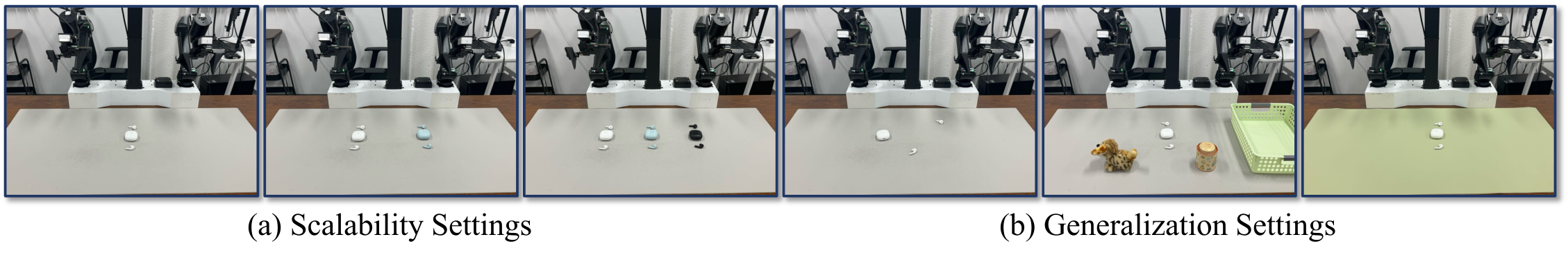
real robot	AC One dual-arm platform, one main camera + two wrist cameras, resolution $320\times240$. The task is earphone packing.Appendix Real Robot Experiments
Main baselines	$\pi_0$, $\pi_{0.5}$, GR00T-N1.5, UWM, DreamZero, Cosmos Policy, GigaWorld-Policy, Motus, Robot4DGen, XR-0, etc.; the appendix explains that some results come directly from relevant benchmark papers.Appendix Baseline Details
Code/Project Page	https: //sharinka0715.github.io/X-WAM/

Complete training configuration table

stage	Hardware	Batch	LR	Steps	Others
Large-scale pretraining	256 NVIDIA H20 GPUs	per-GPU 8, total 2048	$1\times10^{-4}$ peak	40, 000	AdamW; 1000 warmup; cosine decay to 0; $H=8$; $M=10$; $p=0.5$; $\lambda_s=\lambda_a=\lambda_D=1.0$.
Benchmark fine-tuning	32 NVIDIA H20 GPUs	per-GPU 4, total 128	$3\times10^{-5}$	20, 000	Similarly warmup + cosine decay; RoboCasa uses raw actions; RoboTwin 2.0 converts relative actions into absolute end-effector poses and then executes them.
Inference	Single card model not specified	-	-	$T_a=10, T_O=50$	UniPC scheduler; classifier-free guidance scale = 1.0.

Pre-training data table

Dataset	Source	Episodes	Duration h
AgibotWorld-Beta	Real	866, 562	2, 221.5
DROID	Real	74, 734	280.3
InternA1-Aloha	Sim	184, 803	1, 337.3
InternA1-Genie1	Sim	50, 638	174.0
InternA1-Lift2	Sim	231, 018	1, 464.7
RoboCasa MimicGen	Sim	56, 771	282.4
RoboTwin 2.0	Sim	27, 500	113.7
Total	-	1, 492, 026	5, 873.9

5.2 Main results

Policy Evaluation

Benchmark	Method	Result
RoboCasa 24 tasks	$\pi_0$ / GR00T-N1.5	62.5 / 64.1 Avg SR
RoboCasa 24 tasks	UWM / DreamZero / Cosmos Policy	60.8 / 62.4 / 67.1 Avg SR
RoboCasa 24 tasks	X-WAM	79.2 Avg SR
RoboTwin 2.0 clean	Motus best listed baseline	88.7
RoboTwin 2.0 randomized	Motus best listed baseline	87.0
RoboTwin 2.0	X-WAM	89.8 clean / 90.7 randomized

RoboCasa shows that X-WAM outperforms the best-listed baseline Cosmos Policy by 12.1 percentage points. In RoboTwin 2.0, X-WAM is the highest in both clean and randomized columns, and randomized is even higher than clean. This paper emphasizes its generalization performance under randomized settings.

4D Reconstruction and Generation

Method	PSNR↑	SSIM↑	LPIPS↓	AbsRel↓	$\delta_1$↑	CD↓
DreamZero + DA3	21.12	0.7788	0.1580	0.1362	0.8594	0.0680
Robot4DGen	22.67	0.8207	0.1026	0.0736	0.9443	0.0134
X-WAM w/o depth + DA3	23.09	0.8916	0.0548	0.1045	0.9089	0.0401
X-WAM	23.46	0.8942	0.0513	0.0349	0.9738	0.0049

RGB indicators and geometric indicators are improved at the same time. In particular, the point cloud CD dropped from 0.0134 of Robot4DGen to 0.0049, indicating that the depth branch directly contributes to geometric reconstruction.

5.3 Ablation experiment

ablation group	Variant	SR↑	Latency ms↓	key results
Depth architecture	No depth	63.0	1033	No depth/point cloud metrics.
Depth architecture	Sequence concatenation	68.7	1888	Highest quality but significantly increased latency.
Depth architecture	Channel concatenation	64.2	1266	Changing the input distribution, neither SR nor quality is optimal.
Depth architecture	Interleaved branch	67.8	1033	Close to sequence concat quality while maintaining no-depth latency.
Noise schedule	Sync train + Sync infer	66.4	4665	The video quality is high but the action is delayed.
Noise schedule	Decoupled train + Async infer	67.2	1033	Fast, but video/geometry quality drops.
Noise schedule	ANS train + Async infer	67.8	1033	Keep latency low while restoring RGB/depth/point cloud quality.

The author's explanation of depth architecture is: although sequence concatenation is slightly more effective, the attention cost/latency is too high; interleaved branch achieves a compromise while keeping the backbone unaffected by depth tokens. The explanation for ANS is that independent decoupled sampling leads to inconsistent training/inference distributions, while coupled sampling of ANS fixes this.

5.4 Supplementary experiments (from appendix)

RoboCasa per-task

The appendix lists 24 RoboCasa tasks. X-WAM's low-scoring tasks include TurnOffStove 35.0, CoffeeSetupMug 45.0, PnPMicrowaveToCounter 57.0; high-scoring tasks include CloseDrawer 100.0, CloseSingleDoor 96.0, CoffeePressButton 96.0, OpenSingleDoor 96.0.Appendix Detailed Results

RoboTwin 2.0 per-task

The appendix lists the clean/randomized success rates of 50 RoboTwin 2.0 tasks. Among the first 24 tasks, most tasks are close to or reach 90-100 in clean/randomized, such as adjust_bottle 100.0/99.0, click_bell 100.0/100.0, lift_pot 100.0/99.0; there are also lower tasks such as hanging_mug 46.0/55.0.Appendix Detailed Results

Real robot experiment

Appendix Figure: AC One dual-arm robot, main camera and dual wrist cameras, and earphone packing task setup.

Setting	XR-0 Progress / Time	X-WAM Progress / Time
Pack 1 earphone	100.0 (24/24), 54.66s	100.0 (24/24), 41.63s
Pack 2 earphones	79.1 (38/48), 115.44s	93.8 (45/48), 113.25s
Pack 3 earphones	63.9 (46/72), 195.66s	68.0 (49/72), 160.72s
Novel placements	58.3 (14/24), 89.63s	70.8 (17/24), 46.68s
Unseen tablecloth	66.7 (16/24), 65.73s	66.7 (16/24), 62.01s
Unseen distractors	66.7 (16/24), 76.32s	75.0 (18/24), 51.53s

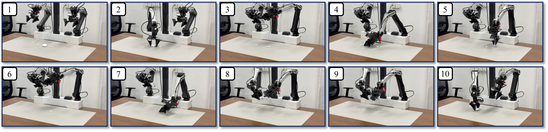
The task is divided into 4 stages: grab the headphone box, open the box lid, grab and insert the headphones, close the lid and put it back on the table; 25% progress for each stage. 6 trials per setting. The author also explained that he had tried to train $\pi_{0.5}$ with the same data, but it did not complete the complete episode and only reached 25%-50% progress in the single-earphone task, so it was not included in the table.Appendix Real Robot Experiments

Appendix Figure: Qualitative rollout of a real AC One dual-arm robot performing earphone packing.

6. Summary of recurrence information

Recurring items	Information given in the paper	Note
Model base	Wan2.2-TI2V-5B video diffusion transformer.	Requires confirmation of base weight licensing, downloadability, and video memory requirements.
Data size	1.49M episodes / 5873.9h.	The cost of fully reproducing pre-training is extremely high; priority should be given to reproducing fine-tuning or small-scale ablation in experiments.
Hardware	Pre-training 256 H20; fine-tuning 32 H20.	The paper clearly gives the training hardware, but does not give a single complete training wall-clock time.
Core hyperparameters	pretrain LR $1e^{-4}$, 40k steps; finetune LR $3e^{-5}$, 20k steps; $T_a=10, T_O=50$; CFG=1.0.	If details such as optimizer betas and weight decay are not listed in the text, they need to be confirmed by the project code.
In-depth supervision	RoboCasa/RoboTwin fine-tuning gains GT depth via simulator replay official demonstrations.	The depth/calibration process of real data must be based on the project materials.
real robot	AC One dual-arm, 1 main camera + 2 wrist cameras, $320\times240$.	reproducibility requires a dual-arm platform and an earphone packing task environment.

7. Analysis, Limitations and Boundaries

7.1 The most valuable part of this paper

Based on the paper's own results, the value of X-WAM lies in pushing unified WAM from 2D video/action joint modeling to 4D RGB-D/action joint modeling, and providing a computationally lighter depth adaptation solution. This design has corresponding experimental support in terms of strategy success rate, RGB quality, depth quality and point cloud geometric indicators.

7.2 Why the results hold up

Wide range of tasks: RoboCasa 24 tasks, RoboTwin 2.0 50 tasks, real-arm earphone packing.
Indicators cover many: Not only policy SR is reported, but also RGB PSNR/SSIM/LPIPS, Depth AbsRel/$\delta_1$, Point Cloud CD.
Ablation directly corresponds to the method module: Depth architecture ablation corresponds to lightweight depth branch; noise schedule ablation corresponds to ANS.
The appendix gives task-level results and training details: Key reproducibility information such as pre-training data, number of GPUs, batch, LR, steps, and inference steps are listed.

7.3 Analysis and explanation of the results given in the paper

The author's explanation of the real robot results is that X-WAM's explicit 3D spatial awareness is more helpful for precise insertion operations and continuous packing stages; the improvement of novel placements especially shows that the model needs to generalize spatial reasoning to unseen object configurations. The author also pointed out that shorter completion time shows that asynchronous denoising with real-time chunking not only reduces inference wait, but may also reduce corrective actions.

7.4 Limitations of the author's statement

Fixed length context: The current framework only handles fixed-length context windows, without historical information or autoregressive rollout; in long-term tasks, if current observations are insufficient to distinguish task stages, it may lead to suboptimal decisions.
Inference latency is higher than dedicated policy: Unified generation of high-dimensional video and low-dimensional actions brings additional latency; the author writes that X-WAM uses 8 denoising steps for about 300 ms per action chunk. Although real-time chunking can overlap computation and execution, the robot may still act based on predictions made several frames ago.

7.5 Applicable boundaries and future work

Applicable boundaries include: tasks require spatial geometry and future world modeling benefits, and can accept higher inference calculations than lightweight VLA; the training end must be able to obtain a large amount of robot data and necessary depth/pose information. The future directions clearly proposed by the author include adding history conditioning, KV caching, autoregressive inference to support a longer temporal horizon, and using distillation, consistency models, or more aggressive asynchronous scheduling to further reduce latency.