Video Prediction Policy: A Generalist Robot Policy with Predictive Visual Representations

arXiv ID：2412.14803, v2, submitted 2024-12-19, revised 2025-05-04

Authors:Yucheng Hu*; Yanjiang Guo*; Pengchao Wang; Xiaoyu Chen; Yen-Jen Wang; Jianke Zhang; Koushil Sreenath; Chaochao Lu; Jianyu Chen

Affiliations:Tsinghua University; UC Berkeley; Shanghai AI Lab; Shanghai Qi Zhi Institute; RobotEra

Publication:ICML 2025 Spotlight Paper

Project page:video-prediction-policy.github.io； Code:roboterax/video-prediction-policy，MIT license

source:arXiv abs, PDF, native LaTeX source, project page, and GitHub README.

One-sentence summary:VPP transforms the video diffusion model from a "slow module that generates complete future videos" to a "predictive visual encoder that only forwards once": first fine-tune Stable Video Diffusion into a manipulation text-guided video prediction model, then extract its internal future representation, use Video Former aggregation and then follow the diffusion transformer policy, allowing the robot strategy to learn implicit inverse dynamics by predicting future visual trajectories.

1. Quick overview of the paper

Introductory items	What does this paper answer?	Where do you focus when reading?
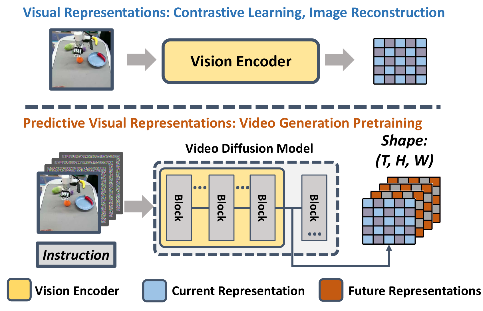
What should the paper solve?	Existing robot vision encoders mostly learn static information from single image reconstruction, double image comparison or image and text comparison, and lack explicit future dynamics; VPP should transform the future prediction representation inside the video diffusion model into the visual conditions of a general robot strategy.	Introduction to the hypothesis of predictive visual representations, and Fig. 1 Comparison of current/future representations.
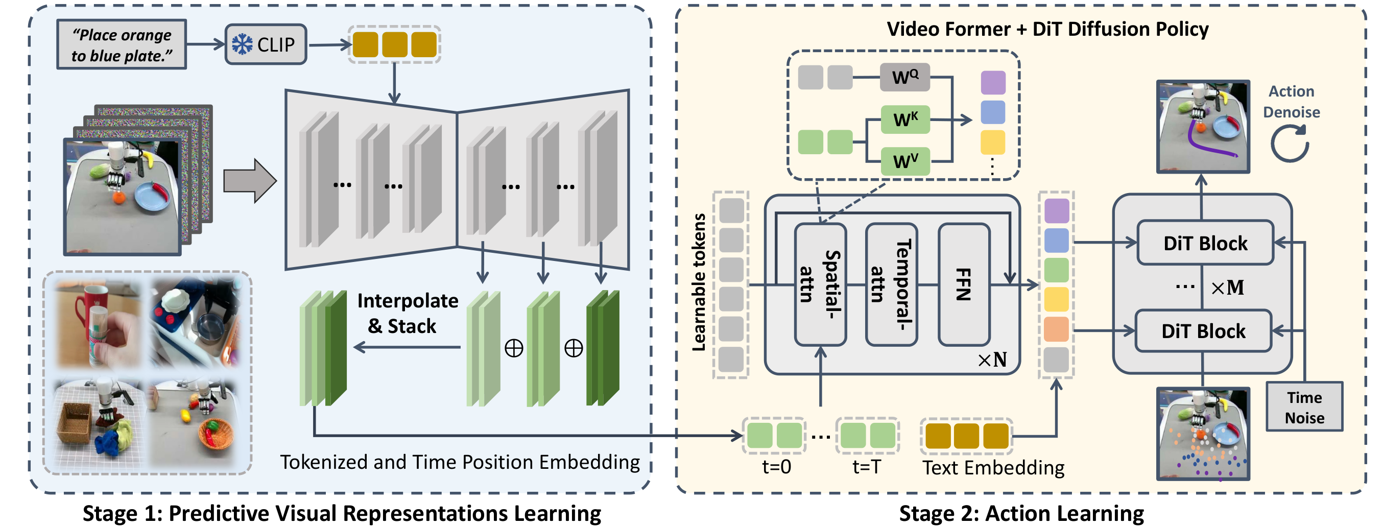
The author's approach	Two stages: first fine-tune SVD to manipulation TVP, then aggregate multi-layer features in TVP forward into predictive representations, output tokens through Video Former, and finally use diffusion transformer policy to generate actions.	Method's TVP objective, feature aggregation, Video Former spatial-temporal attention and diffusion action loss.
most important results	CALVIN ABC-D Avg. Len reaches 4. 33; MetaWorld 50-task average success rate is 0. 682; Panda seen/unseen is 0. 85/0. 73; XHand seen/unseen/tool-use is 0. 75/0. 60/0. 68.	Table 1, MetaWorld table, Table 6, appendix Panda/XHand breakdown table and ablation table.
Things to note when reading	VPP does not rely on complete 30-step video denoising to control the robot, but only uses the internal representation of TVP forward once; this is both the key to high-frequency closed-loop control and the main difference from SuSIE/Uni-Pi/GR-1.	Policy roll-out details, one-step representation of Fig. 5, latency comparison in Video Former and ablation.

Difficulty rating:★★★★☆. Need to understand video diffusion, latent/upsampling features of Stable Video Diffusion, Diffusion Policy/DiT and multi-view spatiotemporal attention. The paper does not have complex theorems, but the method implementation chain is long. During group meetings, it is most likely to be asked "why a forward rough representation of the future is enough to guide actions. "

Numerical caliber reminder:arXiv The summary writing of CALVIN ABC-D is 18. 6% higher than the previous SOTA, corresponding to VPP 4. 33 in Table 1 compared with RoboUniview 3. 65; the introduction and project page writing is 41. 5%, corresponding to the improvement of 3. 06 relative to GR-1. The report explains the two calibers in tables.

1. 1 Contribution list

Propose predictive visual representations:The author believes that the internal latent of VDM contains information about both the current frame and future frames, which is more suitable for sequential control than the visual encoder that only encodes the current observation.
Construct VPP two-stage training:The first stage fine-tunes SVD to manipulation TVP; the second stage trains a generalist action policy conditioned on TVP representations.
High-frequency closed-loop deployment:Incomplete generation of clear video, only one forward representation, combined with Video Former and action chunking, reaches 7-10 Hz on RTX 4090.
Validated across simulation and real platforms:Covers CALVIN, MetaWorld, Franka Panda and XArm+XHand dexterous manipulation.

2. Motivation and related work

2. 1 Why static visual representation is not enough

Robot strategies need to understand "how the world will change next" from the image. Although visual representation learning methods such as R3M, VIP, VC-1, and Voltron can learn semantic and spatial information from video or graphic data, the training goals are usually single image reconstruction, two image comparison, MAE, or language generation, and the model input and output do not explicitly require prediction of the continuous future. These representations are therefore biased toward current states rather than future dynamics.

2. 2 Why video diffusion model is a suitable candidate

The video diffusion model directly models the complete video sequence, and the text-guided video prediction model can also predict future frames based on current observations and language. The author's assumption is that even if future videos are not completely denoised to pixel-level clarity, the intermediate features inside the VDM already contain coarse-grained information about how objects and robots will move. VPP calls these intermediate features predictive visual representations.

Figure 1: VDM internal representation explicitly spans current and future time steps; traditional visual encoders usually only represent the current observation. The core assumption of VPP is that future representations can guide action learning.

2. 3 Differences from future predictive control methods

SuSIE first generates a future goal image and then lets the policy track the image; Uni-Pi learns inverse dynamics between two frames; GR-1 autoregressively generates future frames and actions. The paper believes that these methods have two shortcomings: either they only use a single future prediction and cannot cover complex continuous dynamics; or they require complete denoising/autoregression and low control frequency. The difference of VPP is to use the VDM intermediate representation directly instead of waiting for the final pixel video generation to be completed.

3. Preliminary knowledge

3.1 Video Diffusion Models

$$q(x_t|x_{t-1})=\mathcal{N}(x_t;\sqrt{\alpha_t}x_{t-1},(1-\alpha_t)\mathbb{I}),$$ $$x_t=\sqrt{\bar{\alpha}_t}x_0+\sqrt{1-\bar{\alpha}_t}\epsilon_t,\quad \bar{\alpha}_t=\prod_{i=1}^t\alpha_i.$$

Intuitive understanding:

The forward process continuously adds noise to the real video $x_0$ until it approaches Gaussian noise. Training the video generation model is the reverse process of learning to gradually restore clean video from noisy video.

$$p(x_{t-1}|x_t)=\mathcal{N}\big(x_{t-1};\sqrt{\bar{\alpha}_{t-1}}\mu_\theta(x_t,t),(1-\bar{\alpha}_{t-1})\mathbb{I}\big),$$ $$\mu_\theta(x_t,t)=\frac{x_t-\sqrt{1-\bar{\alpha}_t}\epsilon_\theta(x_t,t)}{\sqrt{\bar{\alpha}_t}}.$$

In text-guided video generation, the model also learns $\epsilon_\theta(x_t,c)$ conditioned on the initial frame and language prompt. VPP subsequently uses this conditional video prediction model as a visual encoder.

3.2 Diffusion Policy

Diffusion policy treats the action sequence $a_i=(\hat{a}_i,\ldots,\hat{a}_{i+m})$ as a denoising object. Compared with unimodal regression, diffusion policy can express multi-modal action distribution. VPP uses a diffusion transformer block in the action head and uses the predicted visual tokens output by Video Former as cross-attention conditions.

4. Detailed explanation of method

Figure 2: VPP two-stage process. First fine-tune the TVP model, then use Video Former to aggregate the TVP internal predictive representations, and finally use the diffusion transformer policy to output the robot action.

4. 1 Stage 1: Training manipulation TVP model

The authors build on the open source Stable Video Diffusion (SVD) with 1. 5B parameters. The original SVD is mainly conditioned on the initial frame $s_0$; VPP adds the CLIP language feature $l_{emb}$, injects language conditions through cross-attention, and sets the output video to $16\times256\times256$ to improve training and inference efficiency. Apart from these changes the main components of SVD are retained.

$$\mathcal{L}_D=\mathbb{E}_{x_0\sim D,\epsilon,t}\left\|V_\theta(x_t,l_{emb},s_0)-x_0\right\|^2,$$

Here $x_0=s_{0:T}$ is the complete video sequence, and $x_t=\sqrt{\bar{\alpha}_t}x_0+\sqrt{1-\bar{\alpha}_t}\epsilon$ is the noise-added video. The model learns to reconstruct the entire future sequence based on initial observations and language.

$$\mathcal{L}_{video}=\lambda_H\mathcal{L}_{D_H}+\lambda_R\mathcal{L}_{D_R}+\lambda_C\mathcal{L}_{D_C}.$$

The three types of data are internet human manipulation, internet robot manipulation and self-collected/downstream data. The appendix gives the sampling proportions of each data set; these weights are used to balance data of different sizes and qualities.

TVP training data	number of trajectories	Sampling ratio
Something-Something-v2	191,642	0.30
RT-1	87,212	0.15
Bridge	23,377	0.15
BC-Z	43,264	0.08
Taco-Play / Jaco-Play	3,603 / 1,085	0.01 / 0.01
CALVIN-ABC / MetaWorld	18,033 / 2,500	0.10 / 0.05
Panda Arm / Dexterous Hand	2,000 / 2,476	0.05 / 0.10
Total	375,192	1.00

Appendix description: 5, 558 items in Bridge and 2, 048 items in Something-Something-v2 are reserved for validation according to Seer settings; 3% of other data sets are reserved for validation.

4. 2 Stage 2: Treat TVP as a forward vision encoder

Fully denoising high-quality video is very slow and results in open-loops or low-frequency domination. The key engineering choice of VPP is to only perform one forward step of TVP to extract features of the internal up-sampling layers without waiting for the final pixel video.

$$L_m=V_\theta(x_{t'},l_{emb},s_0)_{(m)},\quad L_m\in\mathbb{R}^{T\times C_m\times W_m\times H_m}.$$

$m$ represents an up-sampling layer in TVP. The input is the splicing of the current image $s_0$ and the noisy latent $q(x_{t'}|x_0)$; $t'$ usually corresponds to white noise or a latent close to white noise.

$$L'_m=\mathrm{Interpolation}(L_m),\quad L'_m\in\mathbb{R}^{T\times C_m\times W_p\times H_p},$$ $$F_p=\mathrm{concat}\big((L'_0,L'_1,\ldots,L'_m),\mathrm{dim}=1\big).$$

Why aggregate multiple layers:

The final pixel layer contains a lot of texture detail that is irrelevant to control; intermediate upsampling features are often more preserving motion and spatial structure. VPP does not manually select a single layer, but interpolates to the same resolution and then splices it by channel.

For multi-view robots, VPP predicts future representations for static camera and wrist camera respectively, and obtains $F_p^{static}$ and $F_p^{wrist}$. This keeps the input form of TVP simple and allows Video Former to handle multiple views uniformly.

4. 3 Video Former: Compressed spatio-temporal multi-view representation

The predictive representation is a high-dimensional feature sequence of $T\times C\times W\times H$. Video Former uses a fixed number of learnable tokens $Q_{[0:T,0:L]}$ to aggregate these representations. Each frame first performs spatial attention, and then performs temporal attention across time.

$$Q'=\{\mathrm{Spat\text{-}Attn}(Q[i],(F_p^{static}[i],F_p^{wrist}[i]))\}_{i=0}^{T},$$ $$Q''=\mathrm{FFN}(\mathrm{Temp\text{-}Attn}(Q')).$$

The output $Q''$ is fixed-length tokens, which are subsequently used as the cross-attention condition of the diffusion policy.

4.4 Diffusion transformer action head

The action head takes the noised action sequence as input and uses DiT/decoder blocks to gradually restore the action. The aggregated $Q''$ is injected into each transformer block through cross-attention. The goal of motion denoising is:

$$a_k=\sqrt{\bar{\beta}_k}a_0+\sqrt{1-\bar{\beta}_k}\epsilon,$$ $$\mathcal{L}_{\mathrm{diff}}(\psi;A)=\mathbb{E}_{a_0,\epsilon,k}\left\|D_\psi(a_k,l_{emb},Q'')-a_0\right\|^2.$$

Here $a_0$ is the real action sequence, and $D_\psi$ directly predicts the denoised action. VPP also uses action chunking to output multiple action steps to increase control frequency.

5. Intensive reading of experimental results and charts

5. 1 Simulation settings

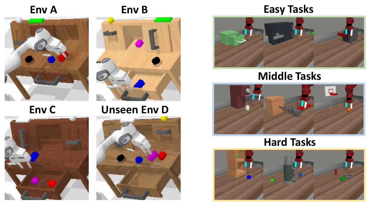
Simulations include CALVIN ABC$\rightarrow$D and MetaWorld. The training environment in CALVIN is ABC, the test environment is unseen D, and only language-annotated ABC data is used for training according to the GR-1 settings. MetaWorld contains 50 Sawyer robot tasks, each task collects 50 trajectories using the official Oracle policy. TVP fine-tuning requires 8 A100s for 2-3 days; policy training requires 4 A100s for 6-12 hours.

Figure 3: CALVIN and MetaWorld task environments, and MetaWorld 50-task success rate table.

5.2 CALVIN ABC-D long-horizon

Category	Method	Data	Task 1	Task 3	Task 5	Avg. Len
Direct action	RT-1	100% ABC	0.533	0.094	0.013	0.90
Direct action	Diffusion Policy	100% ABC	0.402	0.026	0.000	0.56
Future prediction	SuSIE	100% ABC	0.870	0.490	0.260	2.69
Future prediction	GR-1	100% ABC	0.854	0.596	0.401	3.06
Future prediction	VidMan	100% ABC	0.915	0.682	0.467	3.42
3D method	RoboUniview	100% ABC	0.942	0.734	0.507	3.65
Ours	VPP	100% ABC	0.965	0.866	0.769	4.33
Data efficiency	GR-1	10% ABC	0.672	0.198	0.069	1.41
Data efficiency	VPP	10% ABC	0.878	0.632	0.453	3.25

CALVIN is evaluated by completing 5 command tasks in a row. The higher the Avg. Len, the better. The success rate of VPP on the fifth mission is still 0. 769, indicating that the attenuation of long-chain missions is significantly smaller than that of GR-1 and VidMan. VPP's 3. 25 also outperforms multiple full-data future prediction methods in the 10% data setting.

5.3 MetaWorld 50-task

Method	Easy (28)	Middle (11)	Hard (11)	Average
RT-1	0.605	0.042	0.015	0.346
Diffusion Policy	0.442	0.062	0.095	0.279
SuSIE	0.560	0.196	0.255	0.410
GR-1	0.725	0.327	0.451	0.574
VPP	0.818	0.493	0.526	0.682

MetaWorld results are used to demonstrate that VPP is not only applicable to CALVIN long-chain language tasks. On hard tasks, the VPP is 0. 526, which is higher than GR-1's 0. 451; the average success rate ranges from 0. 574 to 0. 682, which the paper claims is 10. 8 percentage points higher than the strongest GR-1 baseline.

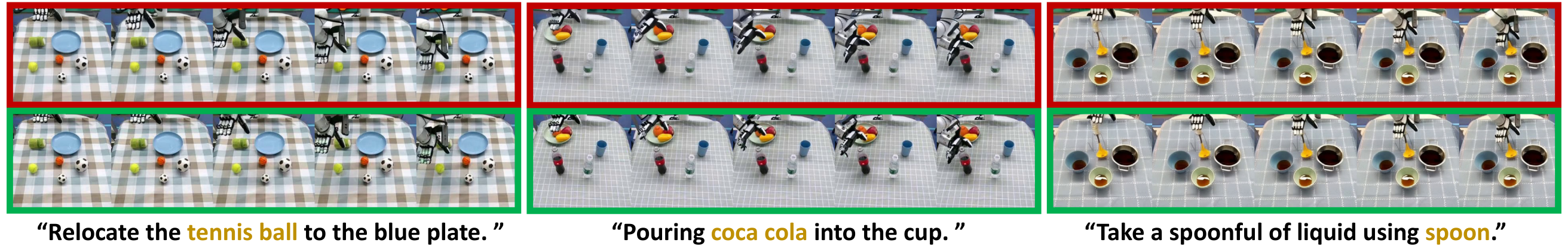
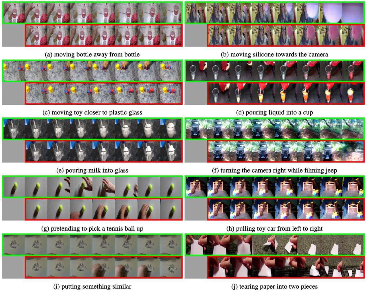
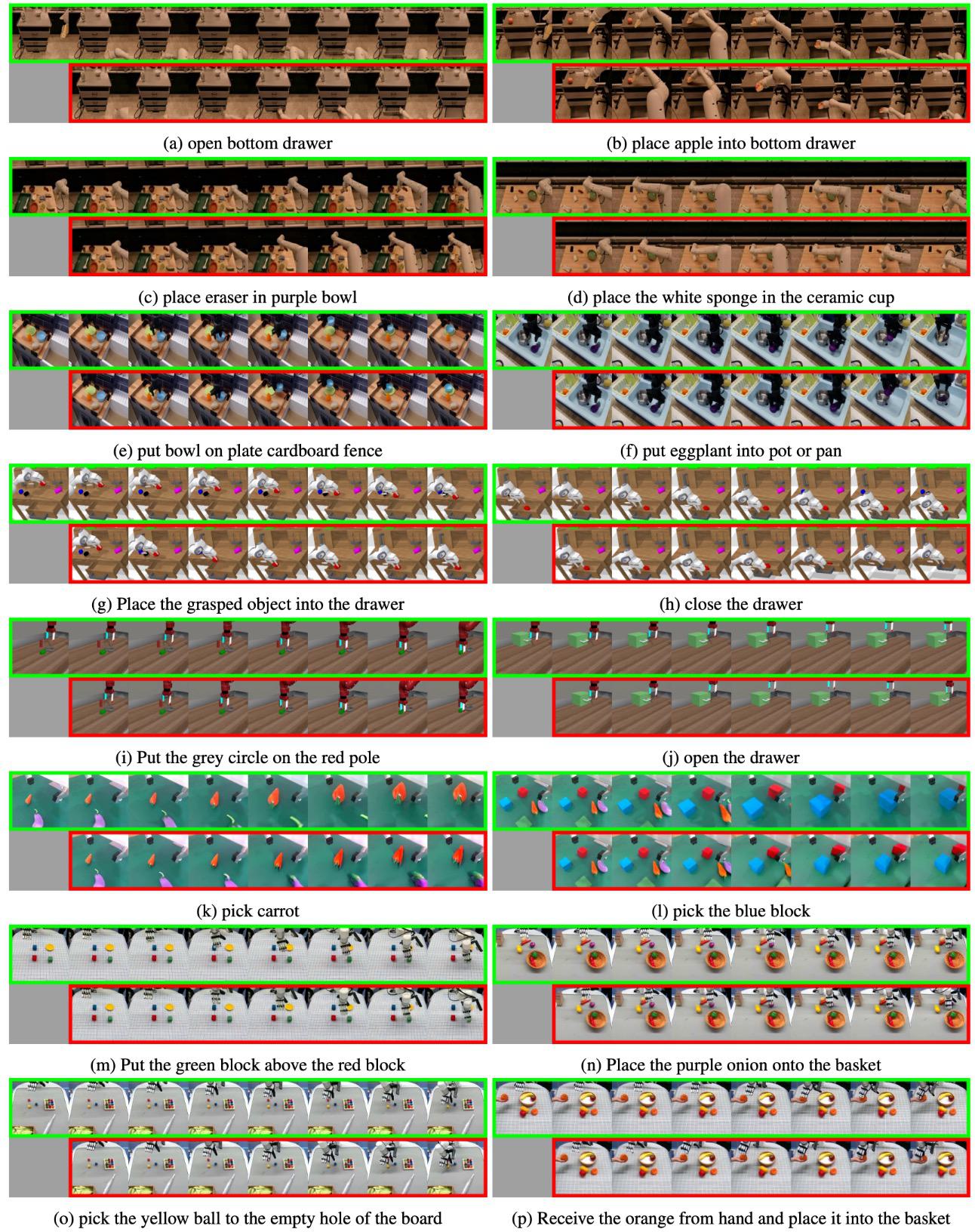
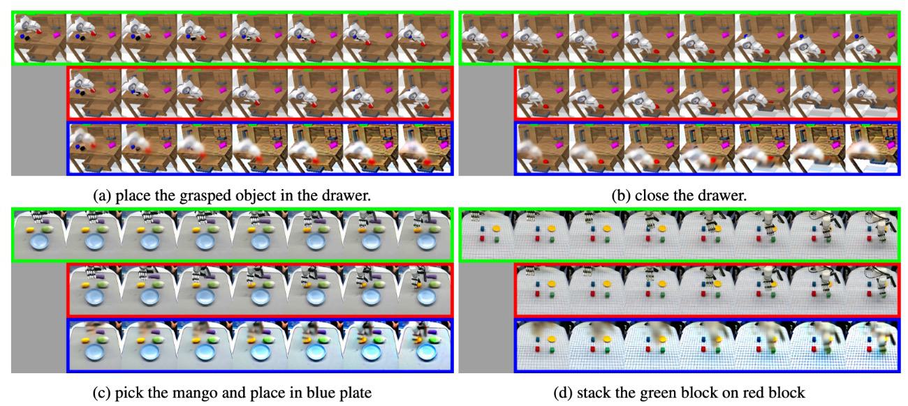
5. 4 Visualization of one-time forward prediction representation

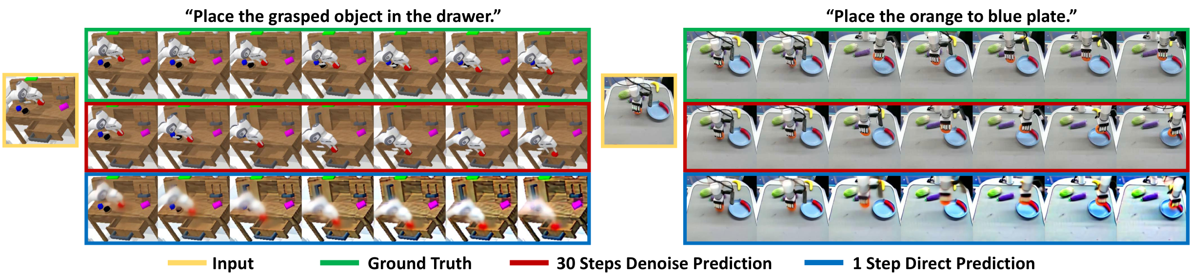
Figure 4: Single-step forward representation compared to full 30-step denoised prediction. Single step means that the texture is not accurate, but it already reflects the movement direction of the object and the robot arm.

This picture is the key to understanding VPP: the author is not saying that one-shot forward can generate beautiful videos, but that it can encode dynamic trends in the intermediate representation that are sufficient to support action learning. The control doesn't need a pixel-perfect future, it just needs to enable the inverse dynamics tracker to track future motion.

5.5 Ablations

Ablation	Avg. Len	Latency	explain
VPP	4.33	about 140 ms	complete model
w/o Internet data	3.97	about 140 ms	Remove internet manipulation co-training
w/o Calvin video	3.31	about 140 ms	Do not fine-tune TVP on downstream CALVIN videos
w/o Internet data + w/o SVD pretrain	1.63	about 140 ms	Training video prediction model from scratch, performance drops significantly
w/o Video Former	3.86	about 450 ms	Accuracy drops and inference slows down
w/o Feature Aggregation	3.60	about 140 ms	Use only final layer features instead of multi-layer aggregation

Visual encoder	Pre-training type	Avg. Len
VDM (VPP)	Video generation	4.33
Stable-VAE	VAE reconstruction	2.58
VC-1	MAE reconstruction	1.23
Voltron	MAE reconstruction + language generation	1.54

More appendix ablation	result
Feature layer	Layer-3 3.72；Layer-6 3.88；Layer-9 4.29；Layer-12 4.05；VPP 4.33
Diffusion time-step	Time-step 10: 4.21；20: 4.33；30: 4.25
Single-view	Avg. Len 3. 58, using only static view; the author points out that this result still exceeds 3. 35 for 3D Diffuser Actor
Ablation 1	Remove the Temporal-attn of Video Former, Avg. Len 4. 18
Ablation 2	TVP is characterized by 2-step denoising, Avg. Len 4. 19, the delay is nearly doubled

5.6 Real-world results

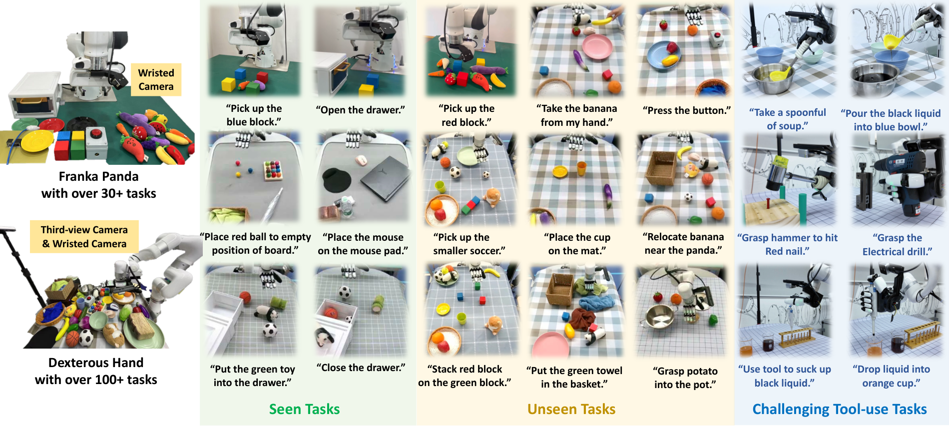
Figure 5: Real hardware platform: Franka Panda arm and XArm + 12-DoF XHand dexterous hand, with some examples of tasks.

The Panda platform collects 2, 000 trajectories, covering 30+ tasks and 6 categories, including picking, placing, pressing, routing, opening, and closing. The XHand platform uses Vision Pro to capture human hand joint motion and retarget it to a 12-DoF dexterous hand; the main text contains 4, 000 items, 100+ tasks, and 13 categories, and the appendix is expressed as 2. 5k trajectories, 100+ tasks, and 10 categories, and additional tool-use tasks are reported. The report is presented separately as main text and appendices. Please note that there is a difference in caliber here.

Platform / setting	Diffusion Policy	SuSIE	GR-1	VPP
Panda seen	0.42	0.56	0.52	0.85
Panda unseen	0.25	0.46	0.38	0.73
XHand seen	0.28	0.45	0.32	0.75
XHand unseen	0.11	0.28	0.15	0.60
XHand tool-use	0.05	0.23	0.15	0.68

The appendix breakdown shows that pick/place/press/route/drawer in Panda unseen are 0. 80/0. 72/0. 80/0. 70/0. 60 respectively. XHand tool-use includes Spoon 0. 9, Hammer 0. 6, Drill 0. 8, Pipette 0. 4, with an average of 0. 68.

Predictions and executions on unseen tasks

Figure 6: Prediction and execution in unseen tasks. Red is the predicted future, and green is the actual execution trajectory; the paper uses this to show that the actual actions will be close to the future predicted by TVP.

5.7 Prediction quality

Appendix reports FVD on Bridge validation: VideoFusion 501. 2, Tune-A-Video 515. 7, Seer 246. 3, VPP 41. 4. The author explains that this improvement comes from using pre-trained SVD as the basis, while early TVP such as Seer did not utilize this video foundation model.

Appendix: 30-step denoising prediction on human manipulation validation.

Appendix: TVP prediction on robotic datasets, green is ground truth, red is predicted future.

Appendix: one-step predictive representations, visualized as blue frames. The authors emphasize that their textures are inaccurate but reflect key physical evolutions.

6. Reproduction list and project details

6. 1 Official code and checkpoints

GitHub README provides PyTorch implementation, the main directories include video_models、policy_models、policy_training、policy_evaluation、video_dataset、video_conf and policy_conf. To reproduce CALVIN, you need to first install the official CALVIN environment and download the ABC-D dataset. The README estimates that the data is about 500 GB.

step	Entrance	illustrate
environment	`conda create -n vpp python==3.10`；`pip install -r requirements.txt`	CALVIN needs to be installed according to mees/calvin; the README mentions that the torch version warning can be ignored.
Video model	`step1_prepare_latent.py` / `step1_train_svd.py`	README is called the main function entry; the file name in the warehouse also contains `step1_prepare_latent.py`。
Action model	`step2_train_action_calvin.py` / `step2_train_action_xbot.py`	Train CALVIN and XBot/XHand strategies separately.
CALVIN evaluation	`policy_evaluation/calvin_evaluate.py`	need `svd-robot-calvin`、`dp-calvin`, CLIP and CALVIN ABC dataset paths.
Video prediction demo	`make_prediction.py --eval --config video_conf/val_svd.yaml ...`	Available at provided `video_dataset_instance` Test prediction on the sample.

README provides Hugging Face checkpoints: CLIP text encoder about 600M;svd-robot About 8G;svd-robot-calvin About 8G;dp-calvin About 1G.

6. 2 Architecture hyperparameters

Type	CALVIN	MetaWorld	Franka Panda	XHand
Video length	16	8	16	16
Action shape	10 x 7	4 x 4	10 x 7	10 x 18
Language shape	20 x 512	20 x 512	20 x 512	20 x 512
Image shape	256 x 256	256 x 256	256 x 256	256 x 256
Video Former token shape	16 x 14 x 384	8 x 28 x 384	14 x 16 x 384	14 x 16 x 384
Video Former input/latent dim	1280 / 512	1280 / 512	1280 / 512	1280 / 512
Video Former heads/layers	8 / 6	8 / 6	8 / 6	8 / 6
Diffusion Transformer latent dim	384	384	384	384
Condition shape	225 x 384	225 x 384	225 x 384	225 x 384
Encoder/decoder layers	4 / 4	4 / 4	4 / 4	4 / 4
Sampling steps	10	10	10	10
TVP batch / policy batch	4 / 76	4 / 64	4 / 128	4 / 128
Epochs / LR	12 / 1e-4	30 / 5e-5	30 / 1e-4	40 / 1e-4

6. 3 Recurrence risk points

Large amount of data:The official CALVIN dataset is about 500 GB, and TVP training also involves multi-source internet/robot/self-collected data.
High training resources:TVP fine-tuning requires 8 A100s for 2-3 days; policy training requires 4 A100s for 6-12 hours.
There is a small difference between the code README and the paper name:mentioned in README step1_prepare_latent_data.py, also in the warehouse list step1_prepare_latent.py; Actual reproduction needs to be checked against the current files in the warehouse.
The core is not to generate clear video:If you focus on the complete 30-step denoising instead of one-step internal features when reproducing, it will deviate from the high-frequency control setting of the paper.
Multi-layer features and timestep need to be set according to the paper:The appendix shows that Layer-9 is close to optimal, diffusion time-step 20 is optimal, and blindly changing layers will affect the results.

7. Analysis, Limitations and Boundaries

7. 1 The most valuable part of this paper

According to the paper's own experimental evidence, the core value of VPP is to rewrite "future prediction" from expensive pixel video generation to a representation extraction problem that can be deployed in a closed-loop. Table 1, Fig. 5 and w/o Video Former/2-step denoising ablation jointly illustrate that the control strategy does not need to wait for clear future video, and only needs a predictive representation of TVP forward, plus Video Former compression, to improve performance and maintain a 7-10 Hz control frequency on CALVIN, MetaWorld and real robot tasks.

7. 2 Why the results hold up

The paper supports the claim through four types of evidence: first, after replacing with Stable-VAE, VC-1, and Voltron, Avg. Len dropped from 4. 33 to 2. 58/1. 23/1. 54, indicating that not any visual encoder can achieve this effect; second, removing internet data, Calvin video, or SVD pretrain all decreased, indicating that video foundation prior and manipulation domain adaptation both contributed; third, layer/time-step/Video Former Ablation explains which designs work; fourth, seen/unseen/tool-use results on real Panda and XHand check for cross-platform generalization.

7. 3 The boundaries of the paper itself that are explicit or exposed by experiments

Requires a strong video basic model and a large amount of video data:When training from scratch and not using SVD pretrain, Avg. Len is only 1. 63, indicating that VPP obviously relies on video foundation prior.
TVP domain adaptation is critical:w/o Calvin video dropped from 4. 33 to 3. 31; w/o Internet data dropped from 4. 33 to 3. 97, indicating that downstream domain video and multi-source data jointly affect the representation quality.
Control frequency depends on one-step encoder design:2-step denoising did not improve performance and almost doubled the inference time; complete video denoising does not comply with the closed-loop control route of the paper.
Real tasks still rely on data alignment within the platform:Although the author emphasizes that internet pretraining helps unseen tasks, real Panda and XHand still collect platform data respectively and train the corresponding generalist policy.
The indicator caliber needs to be distinguished:CALVIN relative improvement uses different baseline calibers in the abstract, text and project pages; Table 1 values should be displayed directly when reporting in group meetings.

7. 4 Group discussion question 1: What is the essential difference between predictive representation and world model?

VPP's TVP will predict future visual sequences, but the policy does not rollout or plan in the prediction world, but uses the internal representation of a forward as a conditional input to learn inverse dynamics. It can be discussed: Is this approach more like representation learning or implicit planning? If it is to be combined with MPC/world-model RL in the future, what state, action, reward or uncertainty structures need to be added?

7. 5 Group meeting discussion question 2: Where does the information of one-step predictive representation come from?

Appendix layer/time-step ablation shows that Layer-9 and time-step 20 are better; Fig. 5 shows that one-step representation is blurry but can express motion. The discussion point is: does this information come from physical priors in SVD pre-training, manipulation TVP fine-tuning, language conditions, or multi-layer feature aggregation? This relates to whether VPP can be transferred to more complex contact, occlusion or long-range tasks.

Suggestions for closing the group meeting:The main line of this paper can be summed up in one sentence: VPP does not require the video model to be "beautifully imagined", but requires it to be "imagined sufficiently controllable" in the internal representation; Video Former and diffusion action head convert this controllable future representation into a closed-loop action.